Mousetracker Data #1
Overview
I'm going to be looking at some pilot data that some colleagues and I collected using Jon Freeman's Mousetracker (http://www.mousetracker.org/). As the name suggests, mousetracker is a program designed to track participants' mouse movements. In social psychology, researchers use it to track participants' implicit decision making processes. Originally, it was developed to study how individuals categorize faces. An example of the paradigm would be a participant having to choose whether a face is male or female, like so: 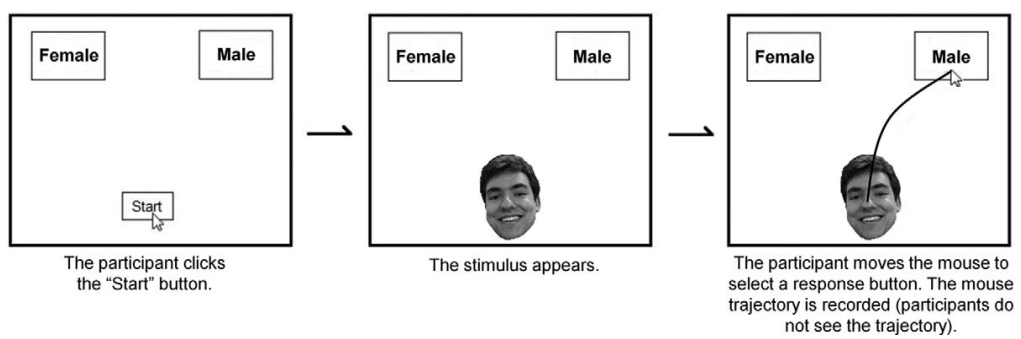
The researcher could then vary the degree to which the face has stereotypically male features, or stereotypically female features, and track not just what participants are categorizing the faces as, but also, how they reach those decisions, by tracking the paths and time course of the mouse movements.
Current project
Anyway, some friends and I are currently working on distinguishing how individuals allocate resources in the context of a relationship. We hypothesize that at any given time, individuals are concerned with:
- their self-interest
- their partner's interests
- the interest of the group or dyad, or the relationship, or them as a pair
and these motives affect the way individuals choose to distribute resources. To distinguish between these three motives, we generated three sets of stimuli using poker chips that pit each of these motives against each other.
The first set of stimuli pit participants' self-interest against the interests of their partner. For example, if red poker chips were paid out to you and green to your partner, one dilemma would be choosing between these two stacks of poker chips of equal height (i.e., the group receives the same in both cases):
| Left | Right |
|---|---|
 |
 |
The second set of stimuli pits a participant's concern for the interest of their partner vs. their own self interest and the group's interest. This captures participants' "pure" altruistic motives in the sense that choosing to favor their partner in this scenario sacrifices both their own interests and the group's interest:
| Left | Right |
|---|---|

|
 |
Finally, the last set of stimuli pit participants' self-interest against that of their partner and the group. In this case, one set of poker chips results in the participant getting more than the other set of chips, but in the other set of poker chips, his/her partner gets more and so does the pair of them:
| Left | Right |
|---|---|

|
 |
The data
The data come in a person-period dataset. This is a "long" format where each participant has multiple rows that represent each trial of the experiment (there were 60 or so trials). However, each row also contains multiple columns each representing a bin of average locations the participant's mouse pointer was during that time span. There are ~100 such bins.
In other words, each participant made 60 choices, and their mouse positions were averaged into ~100 time points per trial.
The first thing we're going to do is to load our data. To do this, we first import Pandas, read our .csv file and print a list of columns. The raw data can be found here: https://raw.githubusercontent.com/bryansim/Python/master/mousetrackerdata/mousetrackercorrected.csv
import pandas as pd
import re
data = pd.read_csv("mousetrackercorrected.csv")
data.columns.values
data.iloc[0:4, 0:19]
Descriptives
In the above data, what we're going to be first doing is finding the mean of participants' reaction time (RT), maximum deviation (MD), and area under curve (AUC). The latter two measures are measures of how much participants were "attracted" to the other option despite selecting the option that they did.
There are two columns for each (e.g., MD_1 and MD_2 depending on which option participants chose). These end up being redundant with one another, and we'll have to combine them.
x-flips and y-flips, as their names suggest, measure the number of times participants' cursors flipped on the x and y axis.
To combine the two MD columns, we create a new column, find all the rows which have data in MD_1, and then fill in the rows which don't have data in MD_1 with the rows that have data in MD_2. We do the same with AUC.
data['MD'] = data.loc[data['MD_1'].isnull() == False, ['MD_1']]
data.loc[data['MD'].isnull() == True,['MD']] = data.loc[data['MD_2'].isnull() == False]['MD_2']
#We do this to get a slice instead of data.loc[data['MD_2'].isnull() == False, ['MD_2']] which returns a dataframe
data['AUC'] = data.loc[data['AUC_1'].isnull() == False, ['AUC_1']]
data.loc[data['AUC'].isnull() == True, ['AUC']] = data.loc[data['AUC_2'].isnull() == False]['AUC_2']
Mean MD and AUC
Now, we can use the .mean() method to get the mean of the above.
data['AUC'].mean()
data['MD'].mean()
Means by choice type
The next thing we want to do is see whether participants differed depending on what the type of choice was (e.g., self vs. other etc.) Eventually, we will have a 3x2 table of means:
| self vs. other | group more w/ self less | group more w/ self more |
|---|---|---|
| chose selfish | chose selfish | chose selfish |
| chose selfless | chose selfless | chose selffless |
Because of the way the conditions were coded (they include trial numbers), we'll use some regex to ignore those numbers:
sodata = data.loc[data['code'].str.extract(r'(so)', expand = False).isnull() == False]
smgldata = data.loc[data['code'].str.extract(r'(smgl)', expand = False).isnull() == False]
smgmdata = data.loc[data['code'].str.extract(r'(smgm)', expand = False).isnull() == False]
print sodata['MD'].mean()
print smgldata['MD'].mean()
print smgmdata['MD'].mean()
print sodata['AUC'].mean()
print smgldata['AUC'].mean()
print smgmdata['AUC'].mean()
AS IT TURNS OUT, this isn't very helpful, because this analysis collapses over whether or not participant chose the selfish or unselfish option, which is really what we're interested in. So let's look at that next:
print sodata.loc[sodata['error'] == 0]['MD'].mean()
print sodata.loc[sodata['error'] == 1]['MD'].mean()
print smgldata.loc[smgldata['error'] == 0]['MD'].mean()
print smgldata.loc[smgldata['error'] == 1]['MD'].mean()
print smgmdata.loc[smgmdata['error'] == 0]['MD'].mean()
print smgmdata.loc[smgmdata['error'] == 1]['MD'].mean()
print sodata.loc[sodata['error'] == 0]['AUC'].mean()
print sodata.loc[sodata['error'] == 1]['AUC'].mean()
print smgldata.loc[smgldata['error'] == 0]['AUC'].mean()
print smgldata.loc[smgldata['error'] == 1]['AUC'].mean()
print smgmdata.loc[smgmdata['error'] == 0]['AUC'].mean()
print smgmdata.loc[smgmdata['error'] == 1]['AUC'].mean()
So, that table above looks like this:
| MD | self vs. other | group more w/ self less | group more w/ self more |
|---|---|---|---|
| chose selfish | .28 | .23 | .18 |
| chose selfless | .29 | .25 | .39 |
| MD | self vs. other | group more w/ self less | group more w/ self more |
|---|---|---|---|
| chose selfish | .51 | .50 | .31 |
| chose selfless | .46 | .37 | .80 |
Note to self: I need to check if I have the selfish vs. selfless options coded correctly. I believe error == 0 = selfish.