Hello!

I'm Bryan. This is my blog of the following projects (links above):

Hack for Heat

In my free time, I volunteer for Heat Seek, an NYC based non-profit that deploys temperature sensors to ensure that everyone in the city has adequate heating over the winter. My posts aim to show some of the groundwork that goes into writing some of our blog posts.

Mediocre Museum

The mediocre part of this project comes from my friend Emilia's and my goal of building the most average artifact possible. We're currently working with open data obtained from the Canada Science and Technology Museums Corporation, obtainable here.
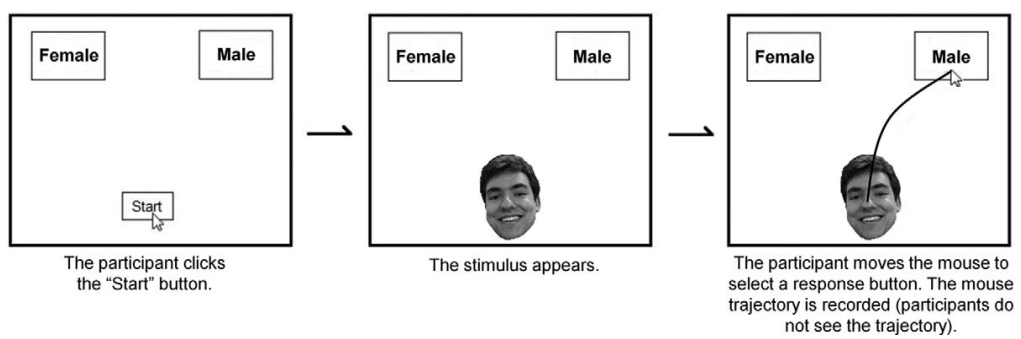
Mousetracker Data

I'm working with my colleagues, Qi Xu and Carlina Conrad, at the NYU Couples Lab to learn more about how people in relationships allocate resources amongsts themselves, and balance self-, altruistic, and group interests.

Skytrax Ratings

What makes a good flight? Using Skytrax ratings data scraped by Quang Nguyen, I'm investigating what factors make up a passenger's overall rating, as well as what influences their decision to recommend an airline to others (vs. not).


Skytrax Data #4: The Logit Model

Skytrax Data #4: The Logit Model

We're going to quickly follow up on the OLS model presented in the last post with an alternative outcome variable: Whether or not passengers chose to recommend the airline to others.

In [1]:
import psycopg2
import pandas as pd
import numpy as np
from sqlalchemy import create_engine
import math
import statsmodels.api as sm
In [2]:
#This connects to the postgres database above.
connection = psycopg2.connect("dbname = skytrax user=skytraxadmin password=skytraxadmin")
cursor = connection.cursor()
In [3]:
connection.rollback()
cursor.execute('SELECT * from airline;')
data = cursor.fetchall()
In [4]:
data = pd.DataFrame(data)
descriptions = [desc[0] for desc in cursor.description]
data.columns = descriptions

In these data, "recommended" is coded as 1 and "not recommended" is coded as 0:

In [25]:
print len(data.loc[data['recommended'] == 1])
print len(data.loc[data['recommended'] == 0])
22098
19298
In [27]:
data.groupby(by = 'recommended').mean()
Out[27]:
overall_rating seat_comfort_rating cabin_staff_rating food_beverages_rating inflight_entertainment_rating ground_service_rating wifi_connectivity_rating value_money_rating
recommended
0 2.640637 2.082208 2.094998 1.773961 1.618873 1.626176 1.403509 1.812525
1 8.327206 3.953765 4.358122 3.667807 3.043509 3.992263 3.547085 4.242555

Unsurprisingly, ratings for flights that are recommended are higher than those that are not.

The logistic regression model

How do these ratings influence whether or not a passenger ultimately choses to recommend an airline to others? To find out, we can calculate the change in odds with each unit change in each variable. For example, for every point higher an airline scores on its overall rating, what is the probability that a passenger selected "1", would recommend, rather than "0"?

Again, we're going to ignore ground service ratings as well as wifi connectivity rating because the vast majority of cases have missing values on these variables.

The first thing we're going to do is center all our predictors. This, as we will see shortly, makes the constant interpretable, and is useful when trying to make point predictions (i.e., what are the odds that someone recommends an airline vs. not if he/she rated it an 8, for example).

In [ ]:
predictors = ['overall_rating', 'seat_comfort_rating', 'cabin_staff_rating', 'food_beverages_rating', \
          'inflight_entertainment_rating', 'value_money_rating']

for predictor in predictors:
    data['{0}_centered'.format(predictor)] = data[predictor] - data[predictor].mean()

I ran two models, one that included passengers' overall ratings, and one that did not:

In [55]:
import statsmodels.api as sm

#x = data[['seat_comfort_rating', 'cabin_staff_rating', 'food_beverages_rating', \
#          'inflight_entertainment_rating', 'value_money_rating']]

x = data[['seat_comfort_rating_centered', 'cabin_staff_rating_centered',\
          'food_beverages_rating_centered', 'inflight_entertainment_rating_centered', 'value_money_rating_centered']]


x = sm.add_constant(x)

logit = sm.Logit(data['recommended'], x, missing = 'drop') #drop missing values

results = logit.fit()
results.summary()
Optimization terminated successfully.
         Current function value: 0.215391
         Iterations 8
Out[55]:
Logit Regression Results
Dep. Variable: recommended No. Observations: 31075
Model: Logit Df Residuals: 31069
Method: MLE Df Model: 5
Date: Tue, 17 May 2016 Pseudo R-squ.: 0.6876
Time: 17:17:33 Log-Likelihood: -6693.3
converged: True LL-Null: -21423.
LLR p-value: 0.000
coef std err z P>|z| [95.0% Conf. Int.]
const 0.0595 0.023 2.610 0.009 0.015 0.104
seat_comfort_rating_centered 0.5314 0.022 24.398 0.000 0.489 0.574
cabin_staff_rating_centered 0.8361 0.021 39.970 0.000 0.795 0.877
food_beverages_rating_centered 0.2134 0.019 11.344 0.000 0.177 0.250
inflight_entertainment_rating_centered 0.0747 0.015 4.915 0.000 0.045 0.105
value_money_rating_centered 1.3341 0.026 52.277 0.000 1.284 1.384
In [56]:
np.exp(results.params)
Out[56]:
const                                     1.061330
seat_comfort_rating_centered              1.701393
cabin_staff_rating_centered               2.307242
food_beverages_rating_centered            1.237909
inflight_entertainment_rating_centered    1.077572
value_money_rating_centered               3.796635
dtype: float64

Interpreting the output

The coefficients of a logistic regression are in log odds, so to make them intuitively interpretable, we exponentiate them to get odds ratios. Odds ratios are simply the likelihood of one case over the other (in our case, it's the likelihood of recommending vs not).

The constant

The constant in this model is the predicted value (in this case, the predicted log odds) when all Xs = 0.

In this case, because we centered our variables at the mean, X=0 refers to the mean of that variable. Thus, our constant in this analysis refers to the odds of recommending vs not recommending for a hypothetical passenger who gave the airline mean ratings across the board. It's value, in this case, 1.06, tells us that this hypothetical passenger was 6% more likely to recommend than not. This is close to the unconditional (i.e., when we don't have any predictors) ratio of 14% (which is what you get when you divide the number of people who recommended vs not).

The coefficients

The coefficients in this model refer to the change in odds with each unit change for each variable. A value above one means that higher passenger ratings on that variable makes it more likely that a passenger recommends an airline. As one might expect, this was the case across the board here.

Let's look at a specific example: The coefficient of value for money, which is the largest here, tells us that, holding all other variables constant (i.e., for our hypothetical passenger that scored an airline the mean for everything), each unit change in value for money made it 3.8 times more likely (than the base rate of 6%) that he/she would recommend vs not.

Including passengers' overall ratings into the model

Next, we're going to look at a model that includes passengers' overall ratings:

In [60]:
#x = data[['overall_rating', 'seat_comfort_rating', 'cabin_staff_rating', 'food_beverages_rating', \
#          'inflight_entertainment_rating', 'value_money_rating']]

x = data[['overall_rating_centered', 'seat_comfort_rating_centered', 'cabin_staff_rating_centered',\
          'food_beverages_rating_centered', 'inflight_entertainment_rating_centered', 'value_money_rating_centered']]

x = sm.add_constant(x)

logit = sm.Logit(data['recommended'], x, missing = 'drop') #drop missing values

results = logit.fit()
results.summary()
Optimization terminated successfully.
         Current function value: 0.128654
         Iterations 9
Out[60]:
Logit Regression Results
Dep. Variable: recommended No. Observations: 28341
Model: Logit Df Residuals: 28334
Method: MLE Df Model: 6
Date: Tue, 17 May 2016 Pseudo R-squ.: 0.8093
Time: 17:32:21 Log-Likelihood: -3646.2
converged: True LL-Null: -19124.
LLR p-value: 0.000
coef std err z P>|z| [95.0% Conf. Int.]
const 0.9089 0.033 27.320 0.000 0.844 0.974
overall_rating_centered 1.2794 0.023 54.786 0.000 1.234 1.325
seat_comfort_rating_centered 0.1691 0.029 5.802 0.000 0.112 0.226
cabin_staff_rating_centered 0.2845 0.029 9.981 0.000 0.229 0.340
food_beverages_rating_centered 0.0528 0.027 1.974 0.048 0.000 0.105
inflight_entertainment_rating_centered 0.0154 0.021 0.726 0.468 -0.026 0.057
value_money_rating_centered 0.5350 0.034 15.784 0.000 0.469 0.601
In [61]:
np.exp(results.params)
Out[61]:
const                                     2.481574
overall_rating_centered                   3.594482
seat_comfort_rating_centered              1.184220
cabin_staff_rating_centered               1.329129
food_beverages_rating_centered            1.054215
inflight_entertainment_rating_centered    1.015530
value_money_rating_centered               1.707426
dtype: float64

Including passengers' overall ratings substantially changed many of the coefficients. Let's go over the different parameters agian:

The constant

The constant for this model is now 2.48, which tells us that the hypothetical passenger who gave the airline the mean score on all ratings is now ~2.5 times more likely to recommend than not (contrast this to 1.06 in the previous model). What this implies is that an "average" in terms of an overall rating is really, on average, an endorsement of the airline.

The coefficients

Here, compared to the previous model, the coefficients for all the other ratings are "depressed", in they are much smaller than before. They are still positive, which means that in general, higher ratings on these criteria = more likely to recommend, but knowing a passenger's overall rating makes that information somewhat redundant.

Summary

In sum, when passengers are made to rate airlines this way, their decision to recommend is dominated by their overall, wholistic rating of the airline. That said, these ratings are all correlated, so the takeaway point should not be that inflight entertainment (which was a non-significant predictor even with an n of 28,000) is unimportant, but rather that further analyses should be done to assess the relative contribution of each predictor to a passenger's overall rating.

Skytrax Data #3: The OLS Model

Skytrax Data #3: The OLS Model

In this post, we're going to examine one way someone might evaluate which rating is the "most important" one in predicting passengers' overall ratings: By examining coefficients in a multiple regression. Recall that besides passengers' overall ratings, there were 7 other criteria: their ratings of the flight's seat comfort, cabin staff, food and beverage, inflight entertainment, ground service, wifi connectivity, and value for money.

In [1]:
import psycopg2
import pandas as pd
import numpy as np
from sqlalchemy import create_engine
import math
import statsmodels.api as sm
In [2]:
#This connects to the postgres database above.
connection = psycopg2.connect("dbname = skytrax user=skytraxadmin password=skytraxadmin")
cursor = connection.cursor()
In [3]:
connection.rollback()
cursor.execute('SELECT * from airline;')
data = cursor.fetchall()
In [4]:
data = pd.DataFrame(data)
descriptions = [desc[0] for desc in cursor.description]
data.columns = descriptions
In [5]:
data.count()
Out[5]:
airline_name                     41396
link                             41396
title                            41396
author                           41396
author_country                   39805
date                             41396
content                          41396
aircraft                          1278
type_traveller                    2378
cabin_flown                      38520
route                             2341
overall_rating                   36861
seat_comfort_rating              33706
cabin_staff_rating               33708
food_beverages_rating            33264
inflight_entertainment_rating    31114
ground_service_rating             2203
wifi_connectivity_rating           565
value_money_rating               39723
recommended                      41396
dtype: int64

In our subsequent analysis, we're going to ignore ground service ratings as well as wifi connectivity rating because, as you can see, these have very limited data.

In [6]:
from pandas.stats.api import ols as olspd

olspd(y= data['overall_rating'], x = data[['seat_comfort_rating', 'cabin_staff_rating',\
                                           'food_beverages_rating', 'inflight_entertainment_rating',\
                                           'value_money_rating']])
C:\Users\dfthd\Anaconda3\envs\python2\lib\site-packages\IPython\core\interactiveshell.py:2885: FutureWarning: The pandas.stats.ols module is deprecated and will be removed in a future version. We refer to external packages like statsmodels, see some examples here: http://statsmodels.sourceforge.net/stable/regression.html
  exec(code_obj, self.user_global_ns, self.user_ns)
Out[6]:
-------------------------Summary of Regression Analysis-------------------------

Formula: Y ~ <seat_comfort_rating> + <cabin_staff_rating>
             + <food_beverages_rating> + <inflight_entertainment_rating> + <value_money_rating>
             + <intercept>

Number of Observations:         28341
Number of Degrees of Freedom:   6

R-squared:         0.7887
Adj R-squared:     0.7887

Rmse:              1.4956

F-stat (5, 28335): 21157.9768, p-value:     0.0000

Degrees of Freedom: model 5, resid 28335

-----------------------Summary of Estimated Coefficients------------------------
      Variable       Coef    Std Err     t-stat    p-value    CI 2.5%   CI 97.5%
--------------------------------------------------------------------------------
seat_comfort_rating     0.4255     0.0097      43.89     0.0000     0.4065     0.4445
cabin_staff_rating     0.6621     0.0094      70.60     0.0000     0.6437     0.6805
food_beverages_rating     0.1660     0.0085      19.63     0.0000     0.1494     0.1826
inflight_entertainment_rating     0.0317     0.0062       5.09     0.0000     0.0195     0.0439
value_money_rating     0.9759     0.0103      94.89     0.0000     0.9557     0.9960
--------------------------------------------------------------------------------
     intercept    -1.5582     0.0254     -61.42     0.0000    -1.6079    -1.5085
---------------------------------End of Summary---------------------------------

First, this tells us that the model with these 5 predictors predicts about 79% of the variance in participants' overall ratings. In addition, the F-test tells us that this percentage is statistically significant, although it has to be said that with such a large sample (n = 28341), this test was probably always going to be significant.

Second, each of the coefficients tell us the change in Y (overall_ratings) for each unit change in that predictor. For example, for each unit change in passengers' seat comfort ratings, passengers overall ratings increased by .43 points.

In the case of passengers' seat comfort ratings, this relationship is statistically significant. In fact, in this analysis, all the predictors are significantly related to passengers' overall ratings.

However, it should be said that statistical significance and practical significance are not the same. From the coefficients, for example, each unit change in passengers' inflight entertainment ratings only increased their overall rating by 0.03, but each unit change in passengers' value for money ratings increased their overall ratings by .98 points.

That said, the coefficients in this analysis are conditional in that they are adjusted for one another. In other words, these coefficients represent what we know about the relationship between passenger ratings of each of the criteria given our knowledge of how they rated the other elements.

Trying to isolate the impact of a single predictor is not as simple as running 5 separate regression models, because the predictors are correlated. We can illustrate this as follows:

In [7]:
import statsmodels.api as sm

predictors = ['seat_comfort_rating', 'cabin_staff_rating', 'food_beverages_rating', 'inflight_entertainment_rating',\
                'value_money_rating']

cleaned_data = data[['overall_rating','seat_comfort_rating', 'cabin_staff_rating', 'food_beverages_rating', 'inflight_entertainment_rating',\
                'value_money_rating']]

cleaned_data = cleaned_data.dropna()

for predictor in predictors:
    #x = sm.add_constant(cleaned_data[predictor])
    model = sm.OLS(cleaned_data[predictor], cleaned_data['overall_rating'])
    results = model.fit()
    print '{0} coefficient: {1}'.format(predictor, results.params[0])
    print '{0} rsquared: {1}'.format(predictor, results.rsquared)
seat_comfort_rating coefficient: 0.485086064206
seat_comfort_rating rsquared: 0.892254153535
cabin_staff_rating coefficient: 0.53019002014
cabin_staff_rating rsquared: 0.911693773785
food_beverages_rating coefficient: 0.452602436575
food_beverages_rating rsquared: 0.852452501199
inflight_entertainment_rating coefficient: 0.374759040658
inflight_entertainment_rating rsquared: 0.710378283952
value_money_rating coefficient: 0.52075902098
value_money_rating rsquared: 0.931569962502

As you can see, the five separate OLS models give us five R2 values that do not add up to 100% of variance explained. This is because the five predictors are correlated. In a future post, we will use Shapley Value Regression to try and tease them apart.

The Average Thing #5: The Average Place pt.2

In [1]:
%matplotlib inline

The Average Thing #5: The average place pt. 2

This is a quick follow up on the last post: We're going to check our math and look at an alternate way of finding the average location: using the Mercator Projection.

Earlier, we saw that the origin of the average object was somewhere in the Hudson Bay in Canada. This seemed at odds with my intuition. I also had a feeling that the reason this result seemed weird was because my mental representation of the earth was not spherical, but cylindrical (e.g., the Mercator Projection).

To demonstrate this, let's test the simple case where we find the point between the middle of Canada and the UK:

In [6]:
canada = country_locations['Canada']
uk = country_locations['England']

#convert to radians
canada = to_radians(canada)
uk = to_radians(uk)
#convert to cartesian
canada = to_cartesian(canada)
uk = to_cartesian(uk)
#find average
averagepoint = ((canada[0]+uk[0])/2, (canada[1]+uk[1])/2, (canada[2]+uk[2])/2)

print to_latlong(averagepoint)
(68.71255890231265, -45.65693500322893)
In [7]:
from IPython.display import IFrame

IFrame('''https://www.google.com/maps/embed?pb=!1m18!1m12!1m3!1d32299245.83742049!2d-81.10312744481017!3d60\
.38924413554626!2m3!1f0!2f0!3f0!3m2!1i1024!2i768!4f13.1!3m3!1m2!1s0x0%3A0x0!2zNjjCsDQyJzQ1LjIiTiA0NcKwMzknM\
jUuMCJX!5e0!3m2!1sen!2sus!4v1462973875452''', width=800, height=600)
Out[7]:

To visualize how this is really the mid point, we can look at that point on a 3D globe (external link):

The above visualization makes it clear how my intuition differed from reality - the shortest distance between the middle of Canada and the UK is not across the Atlantic, but crosses Greenland.

But let's, for a moment, be flat-earthers, and stick to our flat representation of the earth, like we do whenever we use a map or chart. In this case, we simply average the latitude and longitudes of all the points (see: http://www.geomidpoint.com/calculation.html)

In [10]:
latlon_no_na = data.loc[data['GeoLocations'].isnull() == False]['GeoLocations']
latlon_no_na = latlon_no_na[latlon_no_na != '']
        
avelatlon = reduce(lambda x,y: (x[0] + y[0], x[1] + y[1]), latlon_no_na)

avelatlon = (avelatlon[0]/len(latlon_no_na), avelatlon[1]/len(latlon_no_na))
avelatlon
Out[10]:
(49.76023781406744, -68.28145709782275)

Constructing the map this way gives us a point somewhere in Quebec, which is in line with how we might think of the average point if the world was flat:

In [11]:
IFrame('''https://www.google.com/maps/embed?pb=!1m18!1m12!1m3!1d46671329.280431576!2d-113.3722364450685!\
3d44.44153336080491!2m3!1f0!2f0!3f0!3m2!1i1024!2i768!4f13.1!3m3!1m2!1s0x0%3A0x0!2zNDnCsDQ1JzM2LjkiTiA2OM\
KwMTYnNTMuMiJX!5e0!3m2!1sen!2sus!4v1462977105095''', width = 800, height = 600)
Out[11]:

The Average Thing #4: The Average Place pt.1

In [1]:
%matplotlib inline

The Average Thing #4: The average place pt. 1

Today, we're going to take an initial look at finding where the average artifact comes from.

In [2]:
import pandas as pd
import re
import numpy as np
from matplotlib import pyplot as plt
from geopy.geocoders import Nominatim
pd.get_option("display.max_columns")
pd.set_option("display.max_columns", 40)

data = pd.read_csv("cstmc-CSV-en.csv", delimiter = "|", error_bad_lines=False, warn_bad_lines=False)
C:\Users\dfthd\Anaconda3\envs\python2\lib\site-packages\IPython\core\interactiveshell.py:2723: DtypeWarning: Columns (9,10) have mixed types. Specify dtype option on import or set low_memory=False.
  interactivity=interactivity, compiler=compiler, result=result)

We're going to use the GeoPy package to see if we can extract the latitude and longitude data from each of the countries. Let's start with a test case:

In [3]:
geolocator = Nominatim() #Using the service Nominatim
examplecase = data['ManuCountry'][7]
print examplecase
location = geolocator.geocode(examplecase) #Use the geocode method, 
print location.latitude
print location.longitude
United States of America
39.7837304
-100.4458824

Now, with that latitude and longitude, let's see where that takes us. If you imput the coordinates on Google Maps, it points to somewhere in the middle of the U.S. That's good enough for now:

In [4]:
from IPython.display import IFrame
from IPython.core.display import display

IFrame('''https://www.google.com/maps/embed?pb=!1m14!1m8!1m3!1d11800310.147808608!\
2d-107.43346408765365!3d38.054495438444!3m2!1i1024!2i768!4f13.1!3m3!1m2!1s0x0%3A0x0!2zMznCsDQ3JzAx\
LjQiTiAxMDDCsDI2JzQ1LjIiVw!5e0!3m2!1sen!2sus!4v1462918136743''', width = 800, height = 600)
Out[4]:

Next, we're going to do the same for all the countries of origin:

In [5]:
#This simple function takes a string and returns a tuple of the latitude and longitude
def find_lat_long(string):
    geolocator = Nominatim() #Using the service Nominatim
    location = geolocator.geocode(string, timeout=None) #Use the geocode method, 
    return(location.latitude, location.longitude)

import math

#create a dictionary of all the countries
country_locations = {country:"" for country in data['ManuCountry'].unique() if (country != 'Unknown')\
                          and (country != 'unknown') and (type(country) is str)}

#country_locations = {k: find_lat_long(k) for k, v in country_locations.iteritems()}
for k, v in country_locations.iteritems():
    try:
        country_locations[k] = find_lat_long(k)
    except:
        pass
In [6]:
print country_locations
{'Canada': (61.0666922, -107.991707), 'Brazil': (-10.3333332, -53.1999999), 'Qatar': (25.3336984, 51.2295295), 'Italy': (42.6384261, 12.674297), 'Peru': (-6.8699696, -75.0458514), 'Antarctica': (-82.1081819, 34.378236), 'Panama': (8.3096067, -81.3066245), 'Scotland': (56.7861112, -4.1140517), 'Cambodia': (13.5066394, 104.869423), 'France': (46.603354, 1.8883335), 'Great Britain': (54.31536155, -1.91802339480124), 'Bermuda': (32.3018217, -64.7603582), 'Ireland': (52.865196, -7.9794598), 'Wales': (52.2928116, -3.7389299), 'Argentina': (-34.9964962, -64.9672816), 'Norway': (64.574131, 11.5270102892405), 'Thailand': (14.8971921, 100.83273), 'Bangladesh': (24.4768783, 90.2932426), 'Federal Republic of Germany': (45.4185139, -75.6817796429953), 'Slovakia': (48.7411522, 19.4528646), 'Israel': (30.8760272, 35.0015196), 'Australia': (-24.7761085, 134.755), 'Columbia': (2.893108, -73.7845142), 'Indonesia': (-4.7993355, 114.5632032), 'Singapore': (1.2904527, 103.852038), 'Afganistan': (33.0000866, 64.9998468), 'Czechoslovakia': (41.2133453, -98.6228518), 'German Democratic Republic': (19.4347018, -99.2052135855648), 'United States of America': (39.7837304, -100.4458824), 'South America': (-21.0002178, -61.0006564), 'Union of Soviet Socialist Republics': '', 'Guatemala': (15.6356088, -89.8988086), 'Germany': (51.0834196, 10.4234469), 'Chile': (-31.7613364, -71.3187696), 'Martinique': (14.6113732, -60.9620776), 'Belgium': (50.6407351, 4.66696), 'China': (35.000074, 104.999927), 'Haiti': (19.1399952, -72.3570971), 'Hong Kong': (22.2793278, 114.1628131), 'Philippines': (12.7503486, 122.7312101), 'Spain': (40.0028028, -4.0031039), 'Ukraine': (49.4871968, 31.2718321), 'Europe': (51.0000003, 9.9999997), 'Netherlands': (52.2379891, 5.53460738161551), 'Holland': (42.7876022, -86.1090827), 'Pakistan': (30.3308401, 71.247499), 'Denmark': (55.670249, 10.3333283), 'Poland': (52.0977181, 19.0258159), 'Finland': (63.2467777, 25.9209164), 'Mexico': (19.4325301, -99.1332101), 'North America': (51.0000002, -109.0000001), 'Sweden': (59.6749712, 14.5208584), 'Korea': (35.3985008, 127.937111), 'Hungary': (47.1817585, 19.5060937), 'Switzerland': (46.7985624, 8.2319736), 'Honduras': (15.0610686, -84.5978533), 'New Zealand': (-41.500083, 172.8344077), 'Cuba': (23.0131338, -80.8328747), 'Physics': (14.4832485, 121.0269845), 'Jamaica': (18.1850507, -77.3947692), 'Romania': (45.9852129, 24.6859225), 'England': (52.7954791, -0.540240236617432), 'Portugal': (40.033265, -7.8896262), 'South Africa': (-28.8166235, 24.991639), 'Egypt': (26.2540493, 29.2675469), 'Unknown.': (24.9993709, -77.4417422759927), 'Liechtenshtein': (31.9345932, 34.8325777), 'India': (22.3511148, 78.6677428), 'United Kingdom': (54.7023545, -3.2765752), 'Malaysia': (2.3923759, 112.8471939), 'Austria': (47.2000338, 13.199959), 'Trinidad and Tabago': '', 'Republic of Korea': (35.3985008, 127.937111), 'Northern Ireland': (54.65688285, -6.5634352096912), 'Sri Lanka': (7.878, 80.7038245875), 'Japan': (36.5748441, 139.2394179), 'Taiwan': (23.9739374, 120.9820179)}
In [7]:
data['GeoLocations'] = [country_locations.get(x) for x in data['ManuCountry']] 
#we use .get() instead of country_locations[x] to prevent errors when keys are not in the dictionary
In [12]:
data['GeoLocations'][80:100]
Out[12]:
80                          None
81                          None
82                          None
83    (39.7837304, -100.4458824)
84    (39.7837304, -100.4458824)
85                          None
86                          None
87     (61.0666922, -107.991707)
88     (61.0666922, -107.991707)
89    (39.7837304, -100.4458824)
90    (39.7837304, -100.4458824)
91    (39.7837304, -100.4458824)
92    (39.7837304, -100.4458824)
93    (39.7837304, -100.4458824)
94    (39.7837304, -100.4458824)
95    (39.7837304, -100.4458824)
96    (39.7837304, -100.4458824)
97                          None
98                          None
99    (39.7837304, -100.4458824)
Name: GeoLocations, dtype: object

The above process has yielded tuples of latitudes and longitudes where an artifact's country of origin was available, and null where it hasn't. To average this, we're going to have to do some math, because the earth is round and we can't just add the latitudes and longitudes up:

In [9]:
#We're going to have to convert degrees to radians, so let's define a function to do that:

def to_radians(latlong):
    try:
        return (latlong[0]*3.142/180, latlong[1]*3.142/180)
    except:
        pass

#Next, because the earth is round, we have to convert these to cartesian coordinates:
def to_cartesian(latlongradians):
    try:
        x = math.cos(latlongradians[0]) * math.cos(latlongradians[1])
        y = math.cos(latlongradians[0]) * math.sin(latlongradians[1])
        z = math.sin(latlongradians[0])
        return(x,y,z)
    except:
        pass
    
#Finally, we convert back to our original latitude/longitude:
def to_latlong(cartesian):
    try:
        x = cartesian[0]
        y = cartesian[1]
        z = cartesian[2]
        lon = math.atan2(y, x)
        hyp = math.sqrt(x * x + y * y)
        lat = math.atan2(z, hyp)
        return(lat*180/3.142,lon*180/3.142)
    except:
        pass
    
print data['GeoLocations'][90]    
print to_radians(data['GeoLocations'][90])
print to_cartesian(to_radians(data['GeoLocations'][90]))
print to_latlong(to_cartesian(to_radians(data['GeoLocations'][90])))
(39.7837304, -100.4458824)
(0.6944471162044444, -1.75333868056)
(-0.13948924758883874, -0.7556408246036178, 0.6399606972302785)
(39.7837304, -100.4458824)

Looks like this works! Now, let's map it to the entire series:

In [10]:
data['GeoRadians'] = map(to_radians,data['GeoLocations'])
data['GeoCartesian'] = map(to_cartesian, data['GeoRadians'])

#Now, let's average across all the dimensions by reducing:
geo_no_nan = data.loc[data['GeoCartesian'].isnull() == False]['GeoCartesian']

avgcoordinates = reduce(lambda x,y: (x[0] + y[0], x[1] + y[1], x[2] + y[2]), geo_no_nan)
print avgcoordinates
avgcoordinates = (avgcoordinates[0]/len(geo_no_nan), avgcoordinates[1]/len(geo_no_nan), avgcoordinates[2]/len(geo_no_nan))
print avgcoordinates
print to_latlong(avgcoordinates)
(1612.787448314339, -17961.012440354283, 33139.39424219098)
(0.036587737030724564, -0.40746398458154, 0.7518011397956211)
(61.43857821633736, -84.85795258473567)

This procedure says that the location where the average artifact is manufactured is in the Hudson Bay in Canada:

In [11]:
IFrame('''https://www.google.com/maps/embed?pb=!1m18!1m12!1m3!1d9892352.643336799!2d-98.04822081277437\
!3d59.40187990911089!2m3!1f0!2f0!3f0!3m2!1i1024!2i768!4f13.1!3m3!1m2!1s0x0%3A0x0!2zNjHCsDI2JzE4LjkiTiA\
4NMKwNTEnMjguNiJX!5e0!3m2!1sen!2sus!4v1462926074704''', width = 800, height = 600)
Out[11]:

This seems a little strange to me, and I'm definitely going to have to dig deeper in a future post, but I think my math is right, and perhaps I'm just visualizing this in my head wrongly.

The Average Thing #3: Artifacts Over Time

In [1]:
%matplotlib inline

The Average Thing #3: Artifacts over time

In this post, we're going to explore how the number of artifacts that were received over time.

In [2]:
import pandas as pd
import re
import csv
import itertools
import numpy as np
from matplotlib import pyplot as plt
pd.get_option("display.max_columns")
pd.set_option("display.max_columns", 40)

data = pd.read_csv("cstmc-CSV-en.csv", delimiter = "|", error_bad_lines=False, warn_bad_lines=False)
C:\Users\dfthd\Anaconda3\envs\python2\lib\site-packages\IPython\core\interactiveshell.py:2723: DtypeWarning: Columns (9,10) have mixed types. Specify dtype option on import or set low_memory=False.
  interactivity=interactivity, compiler=compiler, result=result)

From the data dictionary, the first four digits of the artifact number reflect the year in which the museum acquired them. How many artifacts did the museum acquire each year?

In [3]:
data['YearObtained'] = data['artifactNumber'].str.extract(r'(\d\d\d\d)', expand=False)
In [4]:
data['YearObtained'].unique()
Out[4]:
array(['1966', '1967', '1968', '1969', '1970', '1971', '1972', '1973',
       '1974', '1975', '1976', '1977', '1978', '1979', '1980', '1981',
       '1982', '1983', '1984', '1985', '1986', '1987', '1988', '1989',
       '1990', '1991', '1992', '1993', '1994', '1995', '1996', '1997',
       '1998', '1999', '2000', '2001', '2002', '2003', '2004', '2005',
       '2006', '2007', '2008', '2009', '2010', '2011', '2012', '2013',
       '2014', '2015'], dtype=object)

Number of objects each year

This is a dataframe/table of the counts of data each attribute has. Besides telling us how many artifacts the museum received that year (in artifactNumber), it also tells us how many of those cases have available data.

In [5]:
data.groupby(by = 'YearObtained').count()
Out[5]:
artifactNumber ObjectName GeneralDescription model SerialNumber Manufacturer ManuCountry ManuProvince ManuCity BeginDate EndDate date_qualifier patent NumberOfComponents ArtifactFinish ContextCanada ContextFunction ContextTechnical group1 category1 subcategory1 group2 category2 subcategory2 group3 category3 subcategory3 material Length Width Height Thickness Weight Diameter image thumbnail
YearObtained
1966 2110 1719 1540 787 193 1629 1537 588 653 1073 432 925 143 2107 1375 422 1124 483 1662 1662 1276 164 164 115 14 14 9 1550 1188 1221 742 57 20 54 1193 1193
1967 1937 1556 1074 1017 543 1402 1290 521 700 849 257 718 51 1937 735 349 749 456 1498 1498 706 67 67 25 2 2 2 1119 845 999 849 8 39 21 1257 1257
1968 2002 1313 938 469 261 1008 918 342 444 442 151 382 94 2002 478 224 385 215 1239 1239 938 46 46 30 3 3 1 943 694 705 490 1 0 6 1185 1185
1969 2793 2065 1798 950 450 1912 1674 610 753 1094 309 986 189 2793 1098 554 1139 689 2002 2002 1655 201 201 170 2 2 2 1809 1555 1549 1154 0 8 78 1934 1934
1970 2041 1529 827 977 790 1494 1128 370 537 464 139 417 123 2041 662 159 358 157 1503 1503 520 59 59 21 1 1 1 825 778 716 629 2 30 39 1253 1253
1971 1143 809 601 408 241 744 659 329 365 317 111 281 99 1143 383 130 227 166 756 756 506 21 21 13 2 2 0 605 539 550 443 3 4 11 678 678
1972 2127 1540 1528 932 286 1439 1143 561 608 723 257 623 169 2127 1495 197 457 278 1442 1442 793 149 149 122 14 14 0 1533 1258 1335 641 73 1 6 1482 1482
1973 1304 894 778 376 214 796 754 305 376 339 60 256 71 1304 740 206 336 234 848 848 685 44 44 31 0 0 0 780 733 749 645 5 1 17 784 784
1974 1226 894 666 505 324 775 713 431 503 365 131 319 123 1226 500 173 314 198 813 813 617 37 37 15 0 0 0 671 543 552 460 1 1 27 881 881
1975 1683 1128 1047 793 224 1097 1006 570 635 671 258 616 111 1683 560 274 812 361 1088 1088 881 38 38 14 4 4 4 1049 604 972 869 0 2 2 1139 1139
1976 1309 882 950 591 371 871 817 373 433 512 125 425 151 1308 697 208 535 352 812 812 684 33 33 21 3 3 2 953 688 759 607 0 3 4 890 890
1977 1419 943 953 522 264 908 848 420 483 440 112 379 154 1419 754 378 464 397 917 917 651 37 37 20 1 1 1 954 633 884 675 1 2 8 970 970
1978 3567 1271 1172 685 364 1214 1127 498 659 612 208 547 231 3567 933 249 699 354 1246 1246 859 101 101 78 2 2 1 1175 813 1027 832 0 0 18 1143 1143
1979 2322 1339 1137 641 259 1233 1175 500 648 508 122 360 154 2322 857 163 536 237 1303 1301 1114 121 121 101 27 27 21 1137 988 1049 838 0 3 65 1234 1234
1980 1633 1187 1023 654 329 1041 981 427 523 556 249 483 153 1633 725 195 466 306 1033 1033 809 91 91 67 1 1 1 1026 951 891 730 0 34 66 960 960
1981 3163 2168 2028 1343 606 2053 1993 911 1241 1131 442 1071 316 3163 1813 236 1692 438 1979 1979 1867 140 140 81 4 4 3 2031 1744 1807 1554 0 3 28 1928 1928
1982 1796 953 915 544 237 931 882 414 537 505 149 422 148 1796 778 244 572 297 926 926 707 142 142 65 3 3 1 920 807 828 605 10 0 22 896 896
1983 1671 775 811 408 234 747 717 332 439 449 112 419 99 1670 683 191 524 236 754 753 595 70 71 54 0 0 0 810 787 759 667 29 2 45 717 717
1984 2546 1332 1305 661 536 1262 1213 570 765 505 95 477 155 2546 1168 303 995 258 1267 1267 865 87 87 68 1 1 1 1308 1217 1310 1149 15 2 40 1355 1355
1985 2780 1346 1377 583 296 1056 993 473 542 487 114 436 106 2780 1100 396 783 371 1011 1011 790 175 175 86 13 13 13 1377 1199 1096 953 21 1 172 991 991
1986 2113 1046 1107 665 322 1030 974 370 496 588 220 520 129 2113 989 473 846 508 1034 1034 700 130 130 79 7 7 6 1108 1111 1119 893 12 1 33 1080 1080
1987 5122 3544 3727 1923 609 2975 3123 1506 1715 1898 411 1154 259 5122 3674 2476 3077 1386 3461 3461 3261 347 347 267 14 14 10 3724 3454 3364 1710 58 2 97 3157 3157
1988 3277 1736 2047 922 280 1779 1672 558 925 1048 348 941 203 3277 1723 1023 1481 783 1800 1800 1587 459 459 366 50 50 27 2046 1997 2002 1623 47 1 183 1579 1579
1989 1371 696 771 454 161 667 631 292 366 514 194 390 49 1371 731 393 581 337 669 669 574 93 93 67 3 3 1 771 707 645 452 11 1 51 630 630
1990 2280 1380 1320 861 146 1255 1200 305 419 510 232 435 106 2280 1332 626 791 336 916 916 728 379 379 126 23 23 20 1317 1128 1337 1057 34 2 159 941 941
1991 2818 2015 2131 895 234 1741 1708 555 630 1429 319 1106 134 2817 1937 635 1718 524 1791 1791 1603 328 328 214 48 48 46 2126 1871 1828 982 373 3 197 1732 1732
1992 4819 3765 3852 1712 608 3618 3012 1274 1340 2792 583 2549 693 4819 3711 1595 3321 1486 3747 3747 1475 303 303 217 57 57 39 3852 3480 3216 2134 72 9 446 3642 3642
1993 1367 1000 978 587 185 854 817 401 484 658 200 410 62 1367 898 467 785 382 925 925 823 184 184 152 23 23 20 978 861 863 437 29 1 35 974 974
1994 2431 1533 1479 952 153 1421 1383 723 790 1120 341 572 115 2431 1344 559 1390 532 1494 1494 809 227 227 206 26 26 25 1479 1371 1355 626 34 2 18 1478 1478
1995 5929 2256 2249 1374 366 2222 2086 768 993 1244 390 939 220 5929 2234 1543 2183 1218 2297 2297 2035 269 269 188 21 21 6 2249 1915 2052 1485 33 3 59 2242 2242
1996 2496 1470 1361 872 279 1402 1338 550 708 950 261 725 132 2496 1323 766 1239 685 1413 1413 1216 381 381 278 31 31 30 1360 1174 1226 851 31 3 111 1381 1381
1997 2966 1748 1776 1090 504 1706 1634 686 949 1194 237 913 203 2966 1715 1234 1663 1098 1745 1745 1003 311 311 268 31 31 29 1775 1463 1439 1096 100 1 245 1900 1900
1998 2641 1904 1905 1340 140 1926 1659 481 619 1369 368 869 201 2641 1883 1406 1773 941 1872 1871 1661 227 227 207 5 5 3 1906 1330 1517 964 18 2 310 2197 2197
1999 1410 849 892 475 107 866 776 343 372 500 257 431 92 1410 831 675 832 585 900 900 789 150 150 138 46 46 46 871 725 684 476 82 1 78 1041 1041
2000 1059 638 801 404 122 656 703 268 336 408 126 263 119 1059 727 439 577 385 774 774 665 117 117 111 13 13 13 801 686 664 499 31 0 50 783 783
2001 2111 1208 1147 498 163 1129 1062 534 585 637 225 481 126 2111 1094 848 973 671 1132 1132 882 216 216 160 7 7 3 1147 919 950 686 42 0 64 1299 1299
2002 3167 2412 2577 1059 354 2259 2187 774 1109 1970 1073 1626 188 3167 2555 2116 2041 1345 2433 2433 2180 377 377 322 42 42 3 2587 2199 1950 1515 26 1 413 2625 2625
2003 2235 1853 1884 730 76 1859 1724 423 453 1225 609 926 100 2234 1879 1480 1703 531 1774 1764 1436 265 265 225 24 24 7 1886 1501 1438 772 124 2 208 1697 1697
2004 5017 4985 4950 4087 181 4746 4763 828 3563 1836 736 1238 73 5017 4989 4270 4844 4033 4863 4863 1802 2808 2808 657 43 43 29 4989 4838 4627 1064 179 7 186 2896 2896
2005 742 742 738 493 167 658 603 241 274 556 173 395 27 742 734 319 592 258 683 683 583 138 138 116 23 23 23 742 681 648 306 203 3 84 700 700
2006 851 851 851 428 52 840 811 95 282 756 70 510 16 851 851 373 718 554 820 820 767 44 44 32 10 10 0 851 774 452 253 71 3 64 462 462
2007 745 745 743 224 78 706 658 148 200 620 287 481 43 745 738 195 690 178 731 730 608 160 160 143 0 0 0 743 686 658 233 179 0 74 483 483
2008 2005 1996 1998 1670 134 1962 1916 1302 1421 613 172 478 69 2005 2001 1419 1760 1412 1983 1982 646 1323 1323 1260 21 21 10 1998 1925 1909 242 145 0 58 1078 1078
2009 861 861 860 432 117 851 823 258 343 687 209 560 64 847 860 562 644 446 818 805 610 239 230 202 6 6 6 861 761 727 466 31 0 78 668 668
2010 1966 1966 1955 593 83 1923 1913 309 421 1784 1155 1642 205 1966 1957 1792 1811 1581 1957 1957 1745 1192 1188 1091 277 277 272 1954 1618 1500 1129 42 1 269 1139 1139
2011 258 258 255 93 28 240 238 90 101 224 28 138 4 258 253 129 177 79 256 256 163 46 45 43 2 2 2 253 226 203 138 27 0 38 235 235
2012 258 258 257 119 19 256 252 115 114 227 23 181 39 258 258 149 234 122 258 230 182 96 96 83 16 16 5 254 207 205 179 3 0 47 249 249
2013 589 589 587 259 54 582 575 164 187 556 85 426 51 588 588 370 573 359 588 588 539 172 172 168 25 25 20 586 516 490 393 1 0 86 516 516
2014 782 782 782 318 27 743 727 157 220 603 82 488 141 782 781 756 568 567 781 773 562 499 499 446 32 32 0 782 615 458 463 1 1 270 144 144
2015 85 85 75 68 6 59 59 4 40 81 1 64 28 85 85 82 74 82 85 85 34 2 2 0 0 0 0 84 78 67 39 0 0 11 0 0
In [6]:
data.groupby(by = 'YearObtained').count()['artifactNumber'].mean()
Out[6]:
2086.86

The mean number of artifacts per year is 2086.6. Let's combine a scatterplot with a fit line to visualize this. I used the examples from here and here.

In [7]:
from scipy.stats import linregress

plt.figure(figsize = (15,10))

meandata = data.groupby(by = 'YearObtained').count()['artifactNumber']
x = pd.to_numeric(meandata.index.values)
y = meandata

print linregress(x,y)

fitline = np.polyfit(x, y, deg=2)

xpoints = np.linspace(min(x),max(x),100);
plt.plot(xpoints, fitline[2] + fitline[1]*xpoints + fitline[0]*xpoints**2 , color = 'red');

plt.scatter(range(min(x),max(x)+1), meandata);
plt.tight_layout()
plt.xticks(size = 20);
plt.yticks(size = 20);
LinregressResult(slope=-17.623769507803122, intercept=37166.973205282113, rvalue=-0.20498455928950232, pvalue=0.15328806044170382, stderr=12.1460638488731)

Some wrong statistics

If you look above, the function method lingress from the package scipy.stats only takes one predictor (x). First, to add in the polynomial term (x2), we're going to use the sm method from the statsmodels.api package.

A glance at these results suggest that that a quadratic model fit the data better than a linear model (R2 of .25 vs. .02).

It should be said, however, that the inference tests (t-tests) from these results violate the assumption of independent errors. If you look at the "warnings" footnote, under [1], correct standard errors assume that the covariance matrix has been properly specified - it hasn't. One assumption that OLS regression makes is that the errors, or residuals of the model are independent - basically, that the points in the model are not related in some other way than the variables you're using to predict the outcome. In our case, that is untrue, as these are time series data, and years that are temporally close to one another will be related to each other.

In the future, I'm going to learn more about the types of models that are appropriate for these data (e.g., an autoregressive model)

In [9]:
import statsmodels.api as sm

x = pd.to_numeric(meandata.index.values).reshape(50,1)
y = np.array(meandata).reshape(50,1)

xpred = np.column_stack((np.ones(50),np.array(x)))
xpredsquared = np.column_stack((xpred,np.array(x**2)))


print sm.OLS(y,xpred,hasconst=True).fit().summary()
print sm.OLS(y,xpredsquared, hasconst=True).fit().summary()
                            OLS Regression Results                            
==============================================================================
Dep. Variable:                      y   R-squared:                       0.042
Model:                            OLS   Adj. R-squared:                  0.022
Method:                 Least Squares   F-statistic:                     2.105
Date:                Sat, 07 May 2016   Prob (F-statistic):              0.153
Time:                        00:51:12   Log-Likelihood:                -426.05
No. Observations:                  50   AIC:                             856.1
Df Residuals:                      48   BIC:                             859.9
Df Model:                           1                                         
Covariance Type:            nonrobust                                         
==============================================================================
                 coef    std err          t      P>|t|      [95.0% Conf. Int.]
------------------------------------------------------------------------------
const       3.717e+04   2.42e+04      1.537      0.131     -1.14e+04  8.58e+04
x1           -17.6238     12.146     -1.451      0.153       -42.045     6.798
==============================================================================
Omnibus:                       17.851   Durbin-Watson:                   1.535
Prob(Omnibus):                  0.000   Jarque-Bera (JB):               21.727
Skew:                           1.365   Prob(JB):                     1.91e-05
Kurtosis:                       4.724   Cond. No.                     2.75e+05
==============================================================================

Warnings:
[1] Standard Errors assume that the covariance matrix of the errors is correctly specified.
[2] The condition number is large, 2.75e+05. This might indicate that there are
strong multicollinearity or other numerical problems.
                            OLS Regression Results                            
==============================================================================
Dep. Variable:                      y   R-squared:                       0.282
Model:                            OLS   Adj. R-squared:                  0.252
Method:                 Least Squares   F-statistic:                     9.248
Date:                Sat, 07 May 2016   Prob (F-statistic):           0.000411
Time:                        00:51:12   Log-Likelihood:                -418.82
No. Observations:                  50   AIC:                             843.6
Df Residuals:                      47   BIC:                             849.4
Df Model:                           2                                         
Covariance Type:            nonrobust                                         
==============================================================================
                 coef    std err          t      P>|t|      [95.0% Conf. Int.]
------------------------------------------------------------------------------
const      -1.291e+07   3.26e+06     -3.956      0.000     -1.95e+07 -6.34e+06
x1          1.299e+04   3278.612      3.962      0.000      6395.437  1.96e+04
x2            -3.2677      0.824     -3.968      0.000        -4.925    -1.611
==============================================================================
Omnibus:                       16.589   Durbin-Watson:                   2.045
Prob(Omnibus):                  0.000   Jarque-Bera (JB):               19.539
Skew:                           1.287   Prob(JB):                     5.72e-05
Kurtosis:                       4.659   Cond. No.                     8.43e+10
==============================================================================

Warnings:
[1] Standard Errors assume that the covariance matrix of the errors is correctly specified.
[2] The condition number is large, 8.43e+10. This might indicate that there are
strong multicollinearity or other numerical problems.

Skytrax Data #2: Shapley Value Regression

Shapley Value Regression

When we have many variables predicting an outcome, how do we know which is the most "important"? In a multiple regression context, one might think, intuitively, that if you threw all the predictors into the same model, the one with the largest coefficient woud be the most important predictor.

If all the predictors were perfectly orthogonal (i.e., completely uncorrelated), this would be true, as the coefficients would not change as a function of which predictors were included/excluded in the model.

However, in most applications (perhaps even the vast majority of real-world cases), predictors are correlated with one another. This results in overlap in the variance that each predictor explains, and confounds simple interpretation of coefficients and R2 statistics with regard to judging how important one predictor is over another. One consequence of predictors being correlated, for example, is that the order in which predictors are entered into the model affects the degree to which they increase R2.

One solution to this problem is, when dealing with multiple predictors, to iterate over all possible orderings of the predictors, and obtain the average importance of each predictor. This procedure is known as Shapley value regression, and is detailed here.

The R package relaimpo does this, but I wanted to work out an analog in Python.

In [2]:
import numpy as np
import itertools

class fit:
    '''
    This creates an instance of the class OLS with attributes coefficients, fitted_values, residuals, and rsquared 
    '''
    def __init__(self, data, outcome, predictors):
        #We do the following so we can call them as attributes
        self.outcome = outcome
        self.predictors = {key: value for (key,value) in [(x, 0) for x in predictors]}
        #Create some dictionaries with all the predictors as keys, and empty lists as values
        self.resultsrsquared = {k:[] for k in predictors} 
        self.resultscoefficients = {k:[] for k in predictors}
        self.results = {k:[] for k in predictors}
        #The above is preferred over dict.fromkeys(list,default) as the default value is shared among all keys, so appending an object
        #will append it to all keys.
        #See: http://stackoverflow.com/questions/23397153/append-value-to-one-list-in-dictionary-appends-value-to-all-lists-in-dictionary
        self.iterate(data, outcome, predictors)
    
    '''
    The method below returns the coefficients from a least-squares regression.
    '''    
    def ols(self, Y, X): #Y is an nx1 vector, X is an nxp matrix
        X_transpose = np.transpose(X)
        X_transpose_X = np.dot(X_transpose, X)
        X_inverse = np.linalg.inv(X_transpose_X)
        X_transpose_Y = np.dot(X_transpose, Y)
               
        self.coefficients = np.dot(X_inverse, X_transpose_Y)
        self.intercept = float(self.coefficients[0])
        self.coefficientslist = list(self.coefficients[1:]) #Change type to list
        
        '''
        The lines below are for calculating R^2.
        '''
        self.fitted_values = np.dot(X, self.coefficients)
        self.residuals = Y - self.fitted_values        
        
        #SStotal
        yty = np.dot(np.transpose(Y),Y)
        j = np.ones((len(Y),len(Y)))
        ytj = np.dot(np.transpose(Y), j)
        ytj = np.dot(ytj,Y)/len(Y)
        sst = yty - ytj
        #SSerror
        sse = np.dot(np.transpose(self.residuals), self.residuals)
        #SSregression
        ssr = sst - sse
        #rsquared
        self.rsquared = ssr/sst
        return self.coefficientslist
        
    def iterate(self,data, outcome, predictors):
        #Create dataset where we remove missing values listwise
        #SOMETHING IS WRONG WITH HOW YOU ARE SELECTING COLUMNS
        Y = np.array(data['{0}'.format(outcome)])
        
        print "Total cases: {0}".format(len(Y))
        
        all_data = np.column_stack((Y, np.ones((len(Y), 1))))
        for bs in predictors:
            all_data =  np.column_stack((all_data, np.array(data[bs])))
        all_data = all_data[~np.isnan(all_data).any(axis=1)]
        Y = all_data[:,0]
        C = all_data[:,1]
        X = all_data[:,2:]
        
        print "Cases after listwise deletion: {0}".format(len(Y))   
        
        '''
        Iterate through all predictors and return the average coefficient for all combinations of predictors
        '''
        for predictor in range(0, len(predictors)): #for each predictor, let's find the average for 1 to n predictors
        
            otherpredictors = [oth for oth in range(0,len(predictors)) if oth != predictor] #list of other predictors
            dictionaryofcoefficients = {n:[] for n in range(1,len(predictors)+1)} # +1 to reflect 1 to n predictors rather than 0 to n-1
            dictionaryofrsquared = {n:[] for n in range(1,len(predictors)+1)}
            
            Xpredictor = np.column_stack((C,X[:,predictor]))

            for npred in range(0,len(predictors)): #from 1 to n-1 other predictors
                ordering = itertools.combinations(otherpredictors, npred)
                for comb in ordering:
                    #do ols for y and our subset of X
                    if len(comb) == 0:
                        dictionaryofcoefficients[npred+1].append(self.ols(Y, Xpredictor)[0]) 
                        dictionaryofrsquared[npred+1].append(self.rsquared)
                    else:
                        Xsub = X[:,list(comb)] #the other predictors are in this matrix
                        Xsub = np.column_stack((Xpredictor,Xsub)) #combine them
                        dictionaryofcoefficients[npred+1].append(self.ols(Y, Xsub)[0]) 
                        dictionaryofrsquared[npred+1].append(self.rsquared)
            
            dictionaryofrsquared.pop(len(predictors)) #because the model with all predictors always has the same R squared
            
            for k,v in dictionaryofcoefficients.iteritems():
                dictionaryofcoefficients[k] = sum(dictionaryofcoefficients[k])/len(dictionaryofcoefficients[k])
                self.resultscoefficients[predictors[predictor]] = dictionaryofcoefficients
            
            for k,v in sorted(dictionaryofrsquared.iteritems(), reverse = True):    
                if k == 1:
                    dictionaryofrsquared[k] = v[0]
                else:
                    dictionaryofrsquared[k] = (sum(dictionaryofrsquared[k])/len(dictionaryofrsquared[k])) 
                    #- (sum(dictionaryofrsquared[k-1])/len(dictionaryofrsquared[k-1]))
                self.resultsrsquared[predictors[predictor]] = dictionaryofrsquared
            
        for k, v in self.resultsrsquared.iteritems():
            self.results[k] = sum(v.values())/len(v.values())
             

As far as I can tell, this code does about 80% of what I want it to. It returns a list of what the average coefficient for each predictor is as a function of how many other predictors are in the model, and also returns the average R2 of the model with N predictors in it. There's still more to do though:

  1. The code runs extremely slow, probably because of the weird nested for-loops I have in there.
  2. The method doesn't actually return the relative importance of each predictor. This has to do with the average change in R2 that each predictor contributes when added to the model. Right now, it just returns the R2 of the whole model.

I'll be working on this in the coming days, but for now, as an example for what does (and does not) work, let's run this on the Skytrax data, and see what happens:

In [3]:
import psycopg2
import pandas as pd
import numpy as np
In [6]:
#get data from postgres database
connection = psycopg2.connect("dbname = skytrax user=skytraxadmin password=skytraxadmin")
cursor = connection.cursor()
cursor.execute("SELECT * from airline")
testdata = cursor.fetchall()
column_names = [desc[0] for desc in cursor.description]
testdata = pd.DataFrame(testdata)
testdata.columns = column_names
In [8]:
import time
import Shapley
reload(Shapley)

start = time.time()

fit = Shapley.fit(testdata, "overall_rating", ['cabin_staff_rating', 'seat_comfort_rating', 'food_beverages_rating', \
                                                    'inflight_entertainment_rating', 'value_money_rating'])

print "\nAverage coefficients with N other predictors in the model:\n"
print fit.resultscoefficients
print "\nAverage Rsquared with N other predictors in the model:\n"
print fit.resultsrsquared
print "\nThis crap took {0}s to run".format(time.time() - start)
Total cases: 41396
Cases after listwise deletion: 28341

Average coefficients with N other predictors in the model:

{'value_money_rating': {1: 1.8649063450094783, 2: 1.5144640753771565, 3: 1.2811039278852754, 4: 1.1094616213211062, 5: 0.97588253839017369}, 'cabin_staff_rating': {1: 1.7220375706163686, 2: 1.2423932090274965, 3: 0.96482096920203941, 4: 0.78336800727344302, 5: 0.66212106011664673}, 'food_beverages_rating': {1: 1.3824000680960342, 2: 0.74574656752576396, 3: 0.41993379259250335, 4: 0.25813695445838092, 5: 0.16598034625130431}, 'seat_comfort_rating': {1: 1.7279134729889485, 2: 1.103370681632768, 3: 0.76087228190797218, 4: 0.55735092810755438, 5: 0.42553696755928527}, 'inflight_entertainment_rating': {1: 0.81813312432369223, 2: 0.25077293584225169, 3: 0.10988060366414072, 4: 0.055685681377817153, 5: 0.031685430819348603}}

Average Rsquared with N other predictors in the model:

{'value_money_rating': {1: 0.70000482291020016, 2: 0.73437848675413542, 3: 0.75769834885876719, 4: 0.77509515934098283}, 'cabin_staff_rating': {1: 0.61108838008392297, 2: 0.68880734158425838, 3: 0.73593199899832795, 4: 0.76760232624119729}, 'food_beverages_rating': {1: 0.41976593597077677, 2: 0.60519081823348375, 3: 0.70695963415469354, 4: 0.7590299721429592}, 'seat_comfort_rating': {1: 0.52806397291997464, 2: 0.64985921373852684, 3: 0.71984029509356728, 4: 0.76190216873812322}, 'inflight_entertainment_rating': {1: 0.1814590593325032, 2: 0.5789830526105908, 3: 0.70255932748876526, 4: 0.75836033918843182}}

This crap took 255.414000034s to run

The Average Thing #2

In [1]:
%matplotlib inline

The Average Thing #2

This time, we're going to take more in depth look at artifacts that are at the museum and what they are made of. The first thing we're going to do is load the data. Because the code for it is the first post, I'm just going to jump straight to the point where we've successfully processed the dimension data (and converted it to standardized numbers).

A deeper dive into object dimensions

In the last post, we found that all of the dimensions appeared to be skewed in that the means were much higher than the medians. Let's plot them to see what those distributions look like.

In [4]:
plt.figure(figsize = (10,6))
plt.hist(data['WeightNUM'].dropna());
In [5]:
plt.figure(figsize = (10,6));
plt.hist(data['LengthNUM'].dropna());
In [6]:
plt.figure(figsize = (10,6));
plt.hist(data['WidthNUM'].dropna(), bins = 100);
In [7]:
plt.figure(figsize = (10,6));
plt.hist(data['HeightNUM'].dropna(), bins = 100);

The graphs above suggest that there is basically a few (perhaps just one) object that is REALLY REALLY big, and that's pulling the mean up. Just for fun, let's find out what that object is.

In [8]:
data.sort_values(['LengthNUM'], ascending = False).iloc[0:3,:]
Out[8]:
artifactNumber ObjectName GeneralDescription model SerialNumber Manufacturer ManuCountry ManuProvince ManuCity BeginDate EndDate date_qualifier patent NumberOfComponents ArtifactFinish ContextCanada ContextFunction ContextTechnical group1 category1 ... Thickness Weight Diameter image thumbnail LengthINT LengthMULT LengthNUM HeightINT HeightMULT HeightNUM WidthINT WidthMULT WidthNUM WeightINT WeightMULT WeightNUM ThicknessINT ThicknessMULT ThicknessNUM
81085 1999.0265.001 Parasail .1 NYLON SAIL/ METAL FITTINGS/ PLASTIC & POLYE... Astra 29 300316 APCO Aviation Ltd. Israel NaN Netanya 1992 NaN NaN NaN 2.0 .1 BLUE, YELLOW AND GREEN NYLON SAIL;.2 PURPLE... PARAGLIDING IS A DEVELOPMENT OF THE SPORT OF H... A PARAGLIDER IS A CROSS BETWEEN A HANG GLIDER ... ORIGINALLY DEVELOPED FROM THE SQUARE PARACHUTE... Aviation Aircraft ... NaN NaN NaN http://source.techno-science.ca/artifacts-arte... http://source.techno-science.ca/artifacts-arte... 112.8 100.0 11280.0 NaN NaN NaN 29.8 100.0 2980.0 NaN NaN NaN NaN NaN NaN
97539 2008.0001.001 Automobile metal, glass, fibre, resin, wood and synthetic... Meteor/Montcalm 5066433 265A 61 Ford Motor Co. of Canada Ltd. Canada Ontario Oakville 1961 NaN NaN NaN 12.0 Automobile has turquoise colour body; white ha... Canadian-built and owned car considered to be ... Owner driven passenger vehicle for general tra... Following WWll, the Ford Motor Co. offered pot... Motorized Ground Transportation Automotive vehicles ... NaN NaN NaN http://source.techno-science.ca/artifacts-arte... http://source.techno-science.ca/artifacts-arte... 5200.0 1.0 5200.0 1405.00 1.0 1405.0 1210.0 1.0 1210.0 NaN NaN NaN NaN NaN NaN
102774 2012.0039.001 Airplane Limited information available at time of catal... Boeing 720-023B 18024 Boeing Airplane Co. United States of America Washington Seattle 1960 NaN NaN NaN 1.0 Red & white colour scheme. Limited information... , C-FETB proved invaluable in validating elect... Used in the testing of selected aircraft compo... , Pratt & Whitney Canada (PWC) bought the Mode... Aviation Aircraft ... NaN NaN NaN NaN NaN 41.4 100.0 4140.0 12.65 100.0 1265.0 39.9 100.0 3990.0 NaN NaN NaN NaN NaN NaN

3 rows × 51 columns

Apparently there is a paraglider that is 112.8 meters long. Let's pull up a picture of this thing. While we're at that, let's also look at this 5200 cm (52m) car. The last item is a Boeing 720. For that, ~40 meters seems reasonable, and it's what's listed on Wikipedia.

In [9]:
print data['image'].iloc[81085]
print data['image'].iloc[97539]
http://source.techno-science.ca/artifacts-artefacts/images/1999.0265.001.aa.cs.png
http://source.techno-science.ca/artifacts-artefacts/images/2008.0001.001.aa.cs.png

I'll be honest, I'm not sure this thing is that long: Also, this looks like a regular car: These just look like very understandable typos, but they also suggest that we should use the median, which is relatively unaffected by these issues.

Using the median dimensions of all the artifacts, we can calculate the average density of the object, and compare it to this table: http://www.psyclops.com/tools/technotes/materials/density.html:

In [10]:
print 22.8*9.4*12 # volume in cm^3
print 16780/(22.8*9.4*12) # density in grams/cm^3
2571.84
6.52451163369

The density of the average artifact is 6.5 g/cm3 or 6500 kg/m3 and is closest to Zirconium, but in general, consistent with some sort of metal. For reference, Aluminium has a density of 2700 kg/m3, Iron, 7870 kg/m3, and Gold, 19320 kg/m3.

Materials

So, what is the average artifact actually made of? There's a materials column that lists a bunch of different materials. Let's find a way extract those strings.

In [11]:
data['material'][50:60]
Out[11]:
50                   metal->steel;glass
51                                  NaN
52    metal->steel;glass;synthetic;wood
53    metal->steel;glass;synthetic;wood
54       metal->steel;metal->brass;wood
55         metal->steel;synthetic;glass
56         metal->steel;synthetic;glass
57         metal->steel;synthetic;glass
58         metal->steel;synthetic;glass
59         metal->steel;synthetic;glass
Name: material, dtype: object

The format for these strings is an arrow -> to represent a subtype of material, and a semi-colon to represent different material. As a first pass, let's extract the different materials into a list:

In [12]:
data['material'].str.findall(r'\w+')[50:60]
Out[12]:
50                     [metal, steel, glass]
51                                       NaN
52    [metal, steel, glass, synthetic, wood]
53    [metal, steel, glass, synthetic, wood]
54        [metal, steel, metal, brass, wood]
55          [metal, steel, synthetic, glass]
56          [metal, steel, synthetic, glass]
57          [metal, steel, synthetic, glass]
58          [metal, steel, synthetic, glass]
59          [metal, steel, synthetic, glass]
Name: material, dtype: object

There's probably a better way of separating sub-types of materials from the materials themselves, but the regex for that is beyond me at the moment, so let's run with this for now: As a quick and dirty way of guesstimating the main material of the average artifact, we can extract the first material in the list.

In [18]:
data['firstmaterial'] = data['material'].str.extract(r'^(\w+)', expand=False)

These are all the unique materials:

In [14]:
data['firstmaterial'].unique()
Out[14]:
array(['paper', 'wood', 'metal', 'glass', nan, 'skin', 'synthetic',
       'fibre', 'resin', 'ceramic', 'stone', 'fluid', 'bone', 'composite',
       'plant', 'animal', 'shell'], dtype=object)

The next thing we want to do is form a dictionary with this list, and then add counts to it.

In [15]:
withmaterials = data.loc[data['firstmaterial'].isnull() == False] #use only rows with data
firstmaterials = dict.fromkeys(withmaterials['firstmaterial'].unique(), 0) #using the dict method .fromkeys(list, default value)

for material in withmaterials['firstmaterial']:
    firstmaterials[material] += 1

firstmaterials
Out[15]:
{'animal': 39,
 'bone': 98,
 'ceramic': 799,
 'composite': 28,
 'fibre': 2117,
 'fluid': 9,
 'glass': 6177,
 'metal': 29370,
 'paper': 14106,
 'plant': 20,
 'resin': 513,
 'shell': 6,
 'skin': 774,
 'stone': 165,
 'synthetic': 7440,
 'wood': 6978}
In [16]:
 #plot a bar graph where the axis goes from 0 to number of dictionary entries, and the values are the countes of those entires
plt.figure(figsize = (15,10))
plt.bar(range(0,len(firstmaterials)), firstmaterials.values(), align='center')
plt.xticks(range(0,len(firstmaterials)),firstmaterials.keys(),rotation = 'vertical', size = 20);
plt.xlim([-1,len(firstmaterials)]);

Here they are as percentages:

In [17]:
total = sum(firstmaterials.values())

for key, value in firstmaterials.iteritems():
    print key, str(round((float(value)/total)*100,2)) + "%"
synthetic 10.84%
fibre 3.08%
stone 0.24%
shell 0.01%
composite 0.04%
ceramic 1.16%
metal 42.79%
fluid 0.01%
resin 0.75%
paper 20.55%
glass 9.0%
wood 10.17%
plant 0.03%
animal 0.06%
skin 1.13%
bone 0.14%

The Average Thing #1

The Average Thing

The Canada Science and Technology Museums Corporation hosts a repository of all the artifacts in its collection here: (http://techno-science.ca/en/data.php). Let's do something interesting with it.

Reading and cleaning data

The data come in either a .csv or .xml format. Let's first try reading the .csv file, because Pandas has native support for that. First, we import all the packages that we might need (e.g., regex), and tell Pandas not to truncate the columns like it usually does.

In [1]:
import pandas as pd
import re
import csv
import itertools
pd.get_option("display.max_columns")
pd.set_option("display.max_columns", 40)

Now, we import the data to a datafram named "data", using Pandas' built-in method .read_csv, specifying the delimiter "|", and telling it not to break when it comes across a bad line, but instead show a bunch of warnings and still continue.

In [2]:
data = pd.read_csv("cstmc-CSV-en.csv", delimiter = "|", error_bad_lines=False, warn_bad_lines=False)
C:\Users\dfthd\Anaconda3\envs\python2\lib\site-packages\IPython\core\interactiveshell.py:2723: DtypeWarning: Columns (9,10) have mixed types. Specify dtype option on import or set low_memory=False.
  interactivity=interactivity, compiler=compiler, result=result)

If you turn the warnings on, it looks like some of the rows of the csv file have extra columns (i.e., they have 37 columns when we only have 36 column names. Because there are multiple missing values, it's not possible to determine what the extra columns represent. Just by eyeballing things, it looks like about ~500 of the 100,000 cases are problematic.

Our two options are to either ignore these cases, or try and read the xml file, which may or may not pay off. My recommendation is that we just move forward and try and get some initial analysis done before backtracking later if we want to.

Here are the first 3 artifacts in the data:

In [3]:
data.head(n = 3)
Out[3]:
artifactNumber ObjectName GeneralDescription model SerialNumber Manufacturer ManuCountry ManuProvince ManuCity BeginDate EndDate date_qualifier patent NumberOfComponents ArtifactFinish ContextCanada ContextFunction ContextTechnical group1 category1 subcategory1 group2 category2 subcategory2 group3 category3 subcategory3 material Length Width Height Thickness Weight Diameter image thumbnail
0 1966.0001.001 Cover PAPER WESTERN CANADA AIRWAYS LTD. NaN Unknown Unknown NaN NaN 1927 NaN NaN NaN 1.0 NaN AT THE TIME IT WAS THE WORLD'S MOST NORTHERNLY... NaN NaN Aviation Commemorative Stamps & coins NaN NaN NaN NaN NaN NaN paper 4.5 cm 2.6 cm NaN NaN NaN NaN http://source.techno-science.ca/artifacts-arte... http://source.techno-science.ca/artifacts-arte...
1 1966.0002.001 Stamp, postage PAPER WESTERN CANADA AIRWAYS LTD. NaN Unknown Unknown NaN NaN 1927 NaN NaN NaN 1.0 PINK & BLACK ON WHITE NaN NaN NaN Aviation Commemorative Stamps & coins NaN NaN NaN NaN NaN NaN paper 3.8 cm 2.7 cm NaN NaN NaN NaN http://source.techno-science.ca/artifacts-arte... http://source.techno-science.ca/artifacts-arte...
2 1966.0003.001 Stamp, postage PAPER NaN NaN Unknown Unknown NaN NaN 1932 NaN NaN NaN 1.0 DARK & PALE BLUE ON WHITE NaN NaN NaN Aviation Commemorative Stamps & coins NaN NaN NaN NaN NaN NaN paper 12.8 cm 8.4 cm NaN NaN NaN NaN http://source.techno-science.ca/artifacts-arte... http://source.techno-science.ca/artifacts-arte...

And here are some cases which have too many columns:

In [4]:
debug = pd.read_csv("cstmc-CSV-en.csv", header=None, delimiter = "|", error_bad_lines=False, skiprows = 37899, nrows=3)
debug
Out[4]:
0 1 2 3 4 5 6 7 8 9 10 11 12 13 14 15 16 17 18 19 20 21 22 23 24 25 26 27 28 29 30 31 32 33 34 35 36
0 1984.1214.001 Engine, airplane NaN LTC1K-4A/LYCOMING T53 LE09281X Avco Lycoming Div. United States of America Connecticut Stratford 1969 NaN circa NaN 1 NaN NaN Converts heat into mechanical power NaN Aviation Motive power NaN NaN NaN NaN NaN NaN NaN NaN NaN NaN NaN NaN NaN NaN NaN NaN http://source.techno-science.ca/artifacts-arte...
1 1984.1215.001 Engine, airplane NaN LTC1K-4A/LYCOMING T53 LE09285X Avco Lycoming Div. United States of America Connecticut Stratford 1969 NaN circa NaN 1 NaN NaN Converts heat into mechanical power NaN Aviation Motive power NaN NaN NaN NaN NaN NaN NaN NaN NaN NaN NaN NaN NaN NaN NaN NaN http://source.techno-science.ca/artifacts-arte...
2 1984.1216.001 Propeller Glass - Fibre HAMILTON STANDARD 337-339-330-325 Hamilton Standard Propeller Div., United Aircr... United States of America Connecticut East hartford 1969 NaN circa NaN 1 NaN NaN Aircraft propeller NaN Aviation Aircraft parts NaN NaN NaN NaN NaN NaN NaN glass;fibre NaN NaN NaN NaN NaN NaN http://source.techno-science.ca/artifacts-arte... http://source.techno-science.ca/artifacts-arte... http://source.techno-science.ca/artifacts-arte...

Recoding dimensions into actual units

The first thing we're going to do is to do convert all the dimensions, which have mixed units (e.g., 16cm and 10m or whatever) into one common unit. To do this, we're going to use regular expressions and loop through the dimension columns.

The other thing that we might want to do is decide what artifacts to actually use. It looks like some of the artifacts are things like documents and paper, and others are really big things like engines.

Dealing with missing data

As you can see from the example cases above, lots of data is missing or unavailable, which is probably to be expected given that not all columns are necessarily relevant to each artifact. However, this forces us to make a decision when trying to summarize data: How do we decide whether to include or exclude artifacts?

For example, the code below subsets data depending on whether or not any of the measurements of their physical dimensions (weight, height, etc.) are missing:

In [5]:
datasub1 = data.loc[data['Length'].isnull() == False]
datasub2 = datasub1.loc[datasub1['Width'].isnull() == False]
datasub3 = datasub2.loc[datasub2['Height'].isnull() == False]
datasub4 = datasub3.loc[datasub3['Weight'].isnull() == False]

Running the code below will list the problem cases with our regex - some have typos in them, others have European style decimal places (thanks Canada!)

In [6]:
subdata = datasub3
subdata = subdata.reset_index(drop = True)

x = 0
badlines = []
for line in subdata['Length']:
    try:
        re.search(r'(\d*\.\d*) .*', line).group(1)
    except:
        badlines.append(subdata.loc[x, ['Length']][0])
    x +=1

print badlines
['610 cm', '12 cm', '210 cm', '254,9 cm', '12,7 cm', '12,7 cm', '71.0\t cm', '81.0\t cm', '61,5 cm', '61,5 cm', '61,5 cm', '61,5 cm', '42.3\t cm', '59,5 cm', '58,0 cm', '176.O cm', '157,5 cm', '18,5 cm', '2,4 cm', '19,5 cm', '32,0 cm', ' cm', '21,0 cm', '30 cm', '58 cm', '5200 cm', '172,0 cm', '26.,0 cm', '26.,0 cm', '43,7 cm', '200,0 cm', '41,5 cm', '180,0 cm', '150 cm', '41,5 cm', '200 cm', '24 cm', '190 cm', '229 cm', '236 cm']

Let's first sub out the commas for decimal places and remove the '\t' characters.

In [7]:
subdata['Length'] = [re.sub(',', '.', x) for x in subdata['Length']]
subdata['Length'] = [re.sub('\t', '', x) for x in subdata['Length']]

AS IT HAPPENS, you can achieve the above using Pandas' built-in string methods, because I am a moron. Below, we use these methods on the "Length" dimension to replace the commas, extract the digits, extract the units, and then replace the units with the numbers to multiply the digits by (i.e., cm = 1, m = 100).

In [8]:
artifactlengths = data['Length'].str.extract(r'(\d*.\d*)', expand=False)
artifactlengths = artifactlengths.str.replace(',', '.')
artifactlengthmultipliers = data['Length'].str.extract(r'.* ([a-zA-Z]*)', expand=False)

Doing this, we've created a vector (i.e., a Pandas series) of floats, and a separate vector of strings that have the units. For the next step, we want to first replace cm and CM with 1, and m and M with 100, and look for the person who used inches and shoot them.

In [9]:
artifactlengthmultipliers.unique()
Out[9]:
array(['cm', nan, 'M', 'in', 'CM', 'm'], dtype=object)

We create a dictionary to use with the .replace method:

In [10]:
unitreplacement = {
    "mm" : .1,
    "MM" : .1,
    "cm" : 1, 
    "CM" : 1,
    "m" : 100,
    "M" : 100,
    "in" : 2.54,
    "kg" : 1,
    "KG" : 1,
    "gm" : .001,
    "tons" : 1000,
    "lbs" : .453
}
artifactlengthmultipliersNUM = artifactlengthmultipliers.replace(unitreplacement)

And then we multiple our numbers by our multipliers, and now we can use the data to find out the average length of all artifacts:

In [11]:
#We have to coerce because our series contains missing values that cannot be typed
artifactlengthincm = pd.to_numeric(artifactlengths, errors = 'coerce') * artifactlengthmultipliersNUM
In [12]:
print artifactlengthincm.mean()
print artifactlengthincm.median()
44.7114966571
22.8

The average length is 44.71 cm, and the median is 22.8 cm.

Functions to extract digits and units

Now that we've done this once with length, we can write some functions to do the above easily with the rest of the dimensions. We also have a function that will take a list of dimensions, and "numberize" all of them.

In [13]:
#These are the above as functions to run on our other dimensions
def extract_digits(series):
    lengths = series.str.extract(r'(\d*.\d*)', expand = False)
    lengths = lengths.str.replace(',' , '.')
    return pd.to_numeric(lengths, errors = 'coerce')

def extract_multipliers(series):
    multipliers = series.str.extract(r'.* ([a-zA-Z]*)', expand = False)
    unitreplacement = {
    "cm" : 1, 
    "CM" : 1,
    "m" : 100,
    "M" : 100,
    "in" : 2.54,
    "kg" : 1,
    "KG" : 1,
    "gm" : .001,
    "tons" : 1000,
    "lbs" : .453
    }
    multipliers = multipliers.replace(unitreplacement)
    return pd.to_numeric(multipliers, errors = 'coerce')

def numberize_dimensions(listofdimensions, data):
    for dimension in listofdimensions:
        data[dimension + "INT"] = extract_digits(data[dimension])
        data[dimension + "MULT"] = extract_multipliers(data[dimension])
        data[dimension + "NUM"] = data[dimension + "INT"] + data[dimension + "MULT"]
In [14]:
#This was some hacky debugging when I manually did a binary search-type thing to find out which row numbers were messed up
#pd.to_numeric(artifactlengths[96050:96100])
#artifactlengths[96050:96100]

Rest of the dimensions

From the above, the average length of all the artifacts in the collection is 44.7cm. Let's find out what the average is for all the other dimensions:

In [15]:
data['HeightINT'] = extract_digits(data['Height'])
data['HeightMULTI'] = extract_multipliers(data['Height'])
data['HeightNUM'] = data['HeightINT'] * data['HeightMULTI']
print data['HeightNUM'].mean()
print data['HeightNUM'].median()
25.8840089939
9.4

The average height is 25.88 cm and the median is 9.4 cm.

In [16]:
data['WidthINT'] = extract_digits(data['Width'])
data['WidthMULTI'] = extract_multipliers(data['Width'])
data['WidthNUM'] = data['WidthINT'] * data['WidthMULTI']
print data['WidthNUM'].mean()
print data['WidthNUM'].median()
24.1553862744
12.0

The average width is 24.16 cm and the median is 12 cm.

Now, we work on weight. Given that the units for weights range from gm to tons, let's go with kg as the unit we'll use, and assume that tons refer to metric tons. There's also a 'cm' there. Something is wrong.

In [17]:
data['Weight'].str.extract('.* (.*)', expand = False).unique()
Out[17]:
array([nan, 'kg', 'cm', 'tons', 'gm', 'lb'], dtype=object)

Below, we extract the indices of cases with "cm" in the weight. There are 13 cases, and some of them look like a misalignment of the columns, but it's impossible to tell which way they are misaligned.

In [18]:
cmtest = data['Weight'].str.extract('(.* cm)', expand=False)
#Here are three
data[cmtest.isnull() == False][0:3]
Out[18]:
artifactNumber ObjectName GeneralDescription model SerialNumber Manufacturer ManuCountry ManuProvince ManuCity BeginDate EndDate date_qualifier patent NumberOfComponents ArtifactFinish ContextCanada ContextFunction ContextTechnical group1 category1 ... category2 subcategory2 group3 category3 subcategory3 material Length Width Height Thickness Weight Diameter image thumbnail HeightINT HeightMULTI HeightNUM WidthINT WidthMULTI WidthNUM
1934 1966.0971.001 Photograph photograph paper; wood frame; glass; paper & c... NaN NaN JARMAN, FRANK LTD. Canada Ontario Ottawa 1941 NaN NaN NaN 1.0 b + w photograph; black frame presented by Frank Learman to Ralph Bell, Dire... display NaN Aviation Archives ... Archives Personal NaN NaN NaN paper->cardboard;wood->;glass->;metal->steel 49.8 cm 38.8 cm NaN NaN 1.9 cm NaN http://source.techno-science.ca/artifacts-arte... http://source.techno-science.ca/artifacts-arte... NaN NaN NaN 38.8 1.0 38.8
1941 1966.0978.001 Photograph photograph paper; glass; plastic frame; steel ... NaN NaN Royal Canadian Air Force Canada Ontario Ottawa 1927 NaN circa NaN 1.0 b + w photograph; caption in white ink; mounte... RCAF Station Ottawa (later Rockcliffe) was the... taken as part of aerial photography survey for... NaN Aviation Archives ... NaN NaN NaN NaN NaN paper->;glass->;synthetic->plastic;metal->steel 45.3 cm 40.0 cm NaN NaN 2.3 cm NaN http://source.techno-science.ca/artifacts-arte... http://source.techno-science.ca/artifacts-arte... NaN NaN NaN 40.0 1.0 40.0
52400 1989.0488.001 Calculator, air navigation plastic; metal swivel at centre - possibly alu... B-24D NaN Consolidated Aircraft Corp. United States of America California San diego 1941 NaN after NaN 2.0 white with black detail; pale yellow rotating ... NaN used to determine gross weight & fore & aft ce... especially useful on bombers because of varyin... Aviation Navigation instruments & equipment ... NaN NaN NaN NaN NaN synthetic->plastic;metal->aluminum - possible 28.0 cm 25.2 cm NaN NaN 1.0 cm NaN http://source.techno-science.ca/artifacts-arte... http://source.techno-science.ca/artifacts-arte... NaN NaN NaN 25.2 1.0 25.2

3 rows × 42 columns

Let's set those cases to NaN, and just ignore them for now:

In [19]:
data.loc[cmtest.isnull() == False,['Weight']] = None
In [20]:
data['WeightINT'] = extract_digits(data['Weight'])
data['WeightMULT'] = extract_multipliers(data['Weight'])
data['WeightNUM'] = data['WeightINT'] * data['WeightMULT']
print data['WeightNUM'].mean()
print data['WeightNUM'].median()
1058.87995356
16.78

The average weight is 1 ton, which may be a problem if we want to fabricate this. However, the median is much lower, which suggests that the distribution is skewed, and this is also true for the other dimensions, let's take a look at that next.

Skytrax Data #1

In [10]:
%matplotlib inline

Skytrax ratings

Following up on this (http://www.quangn.com/exploring-reviews-of-airline-services/) investigation into Skytrax ratings, which are a collection of ratings by made by airline passengers, I wanted to answer some interesting questions I had of my own.

Specifically, what I was interested in is the relative contribution of each of the different metrics (e.g., ground staff, seat comfort, value) to (a) a passenger's overall rating of the airline, and (b) their decision to recommend the airline to another person. Consequently, which criteria should airlines focus on to improve customers' overall perceptions of them (the equivalent of model lift in logit regression)?

Along the way, I thought I'd sate my own curiousity about the following:

  1. How do passenger ratings differ between types of aircraft?
  2. How do passenger ratings differ by cabin class?
  3. How do passenger artings differ depending on where they come from?
  4. How have ratings changed over time?

But first, let's import the data:

In [1]:
import psycopg2
import pandas as pd
import numpy as np
from sqlalchemy import create_engine
from matplotlib import pyplot as plt
import math

I first loaded the data (obtained from https://github.com/quankiquanki/skytrax-reviews-dataset) into a postgres database. Pandas has a very helpful .to_sql() method that makes this easy:

In [ ]:
#This snippet of code loads all the .csv files into a postgres database that I'd set up.
engine = create_engine("postgres://skytraxadmin:skytraxadmin@localhost/skytrax")
databases = ['airline', 'airport', 'seat', 'lounge'] #csv files

for x in databases:
    data = pd.read_csv("{0}.csv".format(x))
    data.to_sql(x, engine, index = False)
In [2]:
#This connects to the postgres database above.
connection = psycopg2.connect("dbname = skytrax user=skytraxadmin password=skytraxadmin")
cursor = connection.cursor()

Ratings by airline

The first thing I was interested in doing was a sanity check to just make sure that I was looking at the same data that the original blog post analyzed (http://www.quangn.com/exploring-reviews-of-airline-services/).

This was the case, although it appears that the original author of that post took only airlines where there were more than 100 ratings, which is what I happened to do.

First, we select the average rating of each airline, as long as that airline has more than 100 ratings. 100 is arbitrary, but if an airline has only a few ratings, the average rating is likely to be extremely variable across samples:

In [4]:
connection.rollback()
cursor.execute("SELECT airline_name, count(airline_name), avg(overall_rating) FROM airline \
               GROUP BY airline_name HAVING count(airline_name) > 100 ORDER BY avg(overall_rating) desc;")
In [5]:
airline_name_data = cursor.fetchall()
column_names = [desc[0] for desc in cursor.description] #column names are stored in the .description attribute
In [8]:
airline_name_data = pd.DataFrame(airline_name_data)
airline_name_data.columns = column_names

Next, we use matplotlib to plot a simple chart of the top 10 rated airlines:

In [13]:
top_ten_airlines = airline_name_data.loc[range(0,9), ['airline_name','avg']]
figure = plt.figure(figsize=(13,8))
bar_x = range(0,9)
plt.bar(range(0,9), top_ten_airlines['avg'], align = 'center')
plt.xticks(range(0,9),top_ten_airlines['airline_name'], rotation ='vertical', fontsize=15)
plt.xlabel('Airline Name',fontsize=15)
plt.ylabel('Rating out of 10', fontsize=15)
plt.yticks(fontsize=15)
print top_ten_airlines #the bar graph does look a little pointless when you can just print out a list of the top 10 airlines.
#but whatever.
         airline_name       avg
0     asiana-airlines  8.348837
1    garuda-indonesia  8.307692
2          air-astana  8.281553
3     bangkok-airways  8.122066
4     indigo-airlines  8.076923
5          korean-air  8.034921
6             eva-air  7.976351
7     aegean-airlines  7.823789
8  singapore-airlines  7.773148

Ratings by aircraft type

The next thing I wanted to do was to see if ratings differed as a function of what aircraft the passenger took.

In [27]:
connection.rollback()
cursor.execute("SELECT aircraft, count(aircraft), avg(overall_rating) AS ovr, \
avg(seat_comfort_rating) AS cmft, avg(inflight_entertainment_rating) AS inft FROM airline \
WHERE aircraft != 'None' GROUP BY aircraft HAVING count(aircraft) >25 ORDER BY avg(overall_rating) asc;")
In [28]:
aircraft_type_data = cursor.fetchall()
column_names = [d[0] for d in cursor.description]
aircraft_type_data = pd.DataFrame(aircraft_type_data)
aircraft_type_data.columns = column_names
In [29]:
aircraft_type_data
Out[29]:
aircraft count ovr cmft inft
0 Boeing 737 47 5.553191 2.829787 2.888889
1 Boeing 747-400 26 5.615385 3.153846 2.720000
2 Boeing 777 48 5.625000 3.354167 3.191489
3 A320 132 5.636364 2.856061 2.333333
4 A330 74 6.189189 3.243243 3.101449
5 Boeing 787 43 6.255814 3.558140 3.275000
6 A319 26 6.307692 3.115385 2.727273
7 A321 45 6.444444 3.444444 2.416667
8 A380 52 7.000000 3.788462 4.115385
9 Boeing 737-800 61 7.278689 3.622951 3.257143
10 Boeing 777-300ER 29 7.517241 4.103448 3.892857
11 A330-300 28 8.250000 4.000000 4.000000

From the above there are only 11 aircraft types that have more than 25 ratings. A couple of aircraft have multiple listings. These appear to be the updated versions of the same aircraft (737-800 vs. 737 and A330-300 vs A330; I assume the generic types are the older models).

There can be many reasons for this, of course. Newer aircraft tend to be more comfortable and reliable. Furthermore, an airline that runs older aircraft may also be associated with other negative experiences that arise because they're struggling. Alternatively, older aircraft may also be associated with "value" airlines, in which case, if customer expectations are commensurately low, these older aircraft may actually be rated more positively. That seems like a future question worth investigaing.

Boeing vs. Airbus

Just for fun, let's compare the average ratings of Boeing vs. Airbus aircraft. We can use regex to select the different rows:

In [30]:
airbus_aircraft = aircraft_type_data.loc[aircraft_type_data['aircraft'].str.contains(r'A.*')]
boeing_aircraft = aircraft_type_data.loc[aircraft_type_data['aircraft'].str.contains(r'Boeing.*')]
print airbus_aircraft.mean()
print boeing_aircraft.mean()
count    59.500000
ovr       6.637948
cmft      3.407932
inft      3.115684
dtype: float64
count    42.333333
ovr       6.307553
cmft      3.437056
inft      3.204230
dtype: float64

Interestingly, even though Boeing aircraft have comparable (or even slightly higher) ratings on "comfort" and "inflight entertainment", Airbus aircraft have higher overall ratings.

Ratings by cabin type

Finally, let's take a look at whether the flying experience is different for the top 1% than it is for the rest of us. As an aside, if you go on Youtube and listen to air traffic controller recordings at JFK, the ATC uses "Top 1%" as a colloquialism for private jets. We go through the same process to import the data:

In [31]:
connection.rollback()
cursor.execute("SELECT avg(overall_rating) AS ovr, avg(seat_comfort_rating) AS seat, avg(cabin_staff_rating) AS cstaff,\
avg(food_beverages_rating) AS food, avg(inflight_entertainment_rating) AS inflight, avg(ground_service_rating) AS gstaff,\
avg(wifi_connectivity_rating) AS wifi, avg(value_money_rating) AS value, cabin_flown, count(*)\
FROM airline GROUP BY cabin_flown;")
In [32]:
data = cursor.fetchall()
column_names = [desc[0] for desc in cursor.description]
In [33]:
data = pd.DataFrame(data)
data.columns = column_names
In [41]:
data['ovr'] = data['ovr']/2 #rescaling the overall rating (out of 10) to be out of 5
In [40]:
data
Out[40]:
ovr seat cstaff food inflight gstaff wifi value cabin_flown count
0 2.111056 2.371125 2.600531 1.936776 1.578055 2.750000 2.000000 2.664648 None 2876
1 2.928374 3.150485 3.406380 2.971567 2.827994 3.644444 3.153846 3.122679 Premium Economy 1510
2 2.987079 2.986317 3.207894 2.646467 2.222536 2.573143 2.066820 3.099697 Economy 29784
3 3.325650 3.740325 3.771536 3.357233 3.002574 3.276316 3.285714 3.340547 First Class 879
4 3.437469 3.616658 3.873538 3.559762 3.046943 3.375000 2.726190 3.556118 Business Class 6347

The last thing we're going to do for now is to compare ratings between passengers who end up recommending the airline to friends vs. those who do not:

In [35]:
connection.rollback()
cursor.execute("SELECT avg(overall_rating)/2 AS ovr, avg(seat_comfort_rating) AS seat, avg(cabin_staff_rating) AS cstaff,\
avg(food_beverages_rating) AS food, avg(inflight_entertainment_rating) AS inflight, avg(ground_service_rating) AS gstaff,\
avg(wifi_connectivity_rating) AS wifi, avg(value_money_rating) AS value, cabin_flown, count(*), recommended \
FROM airline GROUP BY (cabin_flown, recommended) ORDER BY recommended, cabin_flown;")
In [36]:
cabin_recommend_data = cursor.fetchall()
column_names = [desc[0] for desc in cursor.description]
In [37]:
cabin_recommend_data = pd.DataFrame(cabin_recommend_data)
cabin_recommend_data.columns = column_names

The data below suggest a high degree of polarization. One might imagine that people have an implicit "threshold" value that, once crossed, results in a recommendation. Instead, what we find, perhaps unsurprisingly, is that flights that are not recommended are rated a lot worse than those that are recommended.

This is consistent with, but not exclusively because of, a process whereby people judge their flights as "good" or "bad", and then use the rating system to express their satisfaction/disatisfaction with each of the criteria.

In [38]:
cabin_recommend_data
Out[38]:
ovr seat cstaff food inflight gstaff wifi value cabin_flown count recommended
0 1.542186 2.379014 2.442661 2.227797 2.062937 2.086538 1.433333 1.934594 Business Class 1978 0
1 1.279593 2.059694 2.062266 1.728103 1.556541 1.567488 1.384354 1.822827 Economy 13988 0
2 1.392473 2.623693 2.358885 2.003546 1.942029 1.655172 1.500000 1.723473 First Class 312 0
3 1.249601 2.044709 2.166915 1.862891 1.854790 2.250000 2.000000 1.715318 Premium Economy 692 0
4 1.364362 1.574697 1.641992 1.266938 1.165536 2.000000 1.600000 1.441138 None 2328 0
5 4.203916 4.182438 4.527654 4.165486 3.493651 3.995370 3.444444 4.282444 Business Class 4369 1
6 4.140086 3.860673 4.288908 3.497350 2.851571 3.961905 3.500000 4.223123 Economy 15796 1
7 4.276896 4.363813 4.560311 4.101365 3.586826 4.276596 4.000000 4.227513 First Class 567 1
8 4.215159 4.112840 4.485084 3.936446 3.674479 4.151515 3.875000 4.316176 Premium Economy 818 1
9 4.339286 3.904145 4.445596 3.220779 2.369792 5.000000 4.000000 4.390511 None 548 1

Mousetracker Data #1

Overview

I'm going to be looking at some pilot data that some colleagues and I collected using Jon Freeman's Mousetracker (http://www.mousetracker.org/). As the name suggests, mousetracker is a program designed to track participants' mouse movements. In social psychology, researchers use it to track participants' implicit decision making processes. Originally, it was developed to study how individuals categorize faces. An example of the paradigm would be a participant having to choose whether a face is male or female, like so: mousetracker image here

The researcher could then vary the degree to which the face has stereotypically male features, or stereotypically female features, and track not just what participants are categorizing the faces as, but also, how they reach those decisions, by tracking the paths and time course of the mouse movements.

Current project

Anyway, some friends and I are currently working on distinguishing how individuals allocate resources in the context of a relationship. We hypothesize that at any given time, individuals are concerned with:

  1. their self-interest
  2. their partner's interests
  3. the interest of the group or dyad, or the relationship, or them as a pair

and these motives affect the way individuals choose to distribute resources. To distinguish between these three motives, we generated three sets of stimuli using poker chips that pit each of these motives against each other.

The first set of stimuli pit participants' self-interest against the interests of their partner. For example, if red poker chips were paid out to you and green to your partner, one dilemma would be choosing between these two stacks of poker chips of equal height (i.e., the group receives the same in both cases):

Left Right
so1 so2

The second set of stimuli pits a participant's concern for the interest of their partner vs. their own self interest and the group's interest. This captures participants' "pure" altruistic motives in the sense that choosing to favor their partner in this scenario sacrifices both their own interests and the group's interest:

Left Right
smgm1 smgm2

Finally, the last set of stimuli pit participants' self-interest against that of their partner and the group. In this case, one set of poker chips results in the participant getting more than the other set of chips, but in the other set of poker chips, his/her partner gets more and so does the pair of them:

Left Right
slgm1 slgm2

The data

The data come in a person-period dataset. This is a "long" format where each participant has multiple rows that represent each trial of the experiment (there were 60 or so trials). However, each row also contains multiple columns each representing a bin of average locations the participant's mouse pointer was during that time span. There are ~100 such bins.

In other words, each participant made 60 choices, and their mouse positions were averaged into ~100 time points per trial.

The first thing we're going to do is to load our data. To do this, we first import Pandas, read our .csv file and print a list of columns. The raw data can be found here: https://raw.githubusercontent.com/bryansim/Python/master/mousetrackerdata/mousetrackercorrected.csv

In [1]:
import pandas as pd
import re
In [2]:
data = pd.read_csv("mousetrackercorrected.csv")
data.columns.values
Out[2]:
array(['subject', 'trial', 'stimfile', 'condition', 'code', 'resp_1',
       'resp_2', 'response', 'distractor', 'error', 'init time', 'RT',
       'MD_1', 'MD_2', 'AUC_1', 'AUC_2', 'MD_time', 'x-flip', 'y-flip',
       'z-MD-separate', 'z-MD-together', 'z-AUC-separate',
       'z-AUC-together', 'comments', 'X_1', 'X_2', 'X_3', 'X_4', 'X_5',
       'X_6', 'X_7', 'X_8', 'X_9', 'X_10', 'X_11', 'X_12', 'X_13', 'X_14',
       'X_15', 'X_16', 'X_17', 'X_18', 'X_19', 'X_20', 'X_21', 'X_22',
       'X_23', 'X_24', 'X_25', 'X_26', 'X_27', 'X_28', 'X_29', 'X_30',
       'X_31', 'X_32', 'X_33', 'X_34', 'X_35', 'X_36', 'X_37', 'X_38',
       'X_39', 'X_40', 'X_41', 'X_42', 'X_43', 'X_44', 'X_45', 'X_46',
       'X_47', 'X_48', 'X_49', 'X_50', 'X_51', 'X_52', 'X_53', 'X_54',
       'X_55', 'X_56', 'X_57', 'X_58', 'X_59', 'X_60', 'X_61', 'X_62',
       'X_63', 'X_64', 'X_65', 'X_66', 'X_67', 'X_68', 'X_69', 'X_70',
       'X_71', 'X_72', 'X_73', 'X_74', 'X_75', 'X_76', 'X_77', 'X_78',
       'X_79', 'X_80', 'X_81', 'X_82', 'X_83', 'X_84', 'X_85', 'X_86',
       'X_87', 'X_88', 'X_89', 'X_90', 'X_91', 'X_92', 'X_93', 'X_94',
       'X_95', 'X_96', 'X_97', 'X_98', 'X_99', 'X_100', 'X_101', 'Y_1',
       'Y_2', 'Y_3', 'Y_4', 'Y_5', 'Y_6', 'Y_7', 'Y_8', 'Y_9', 'Y_10',
       'Y_11', 'Y_12', 'Y_13', 'Y_14', 'Y_15', 'Y_16', 'Y_17', 'Y_18',
       'Y_19', 'Y_20', 'Y_21', 'Y_22', 'Y_23', 'Y_24', 'Y_25', 'Y_26',
       'Y_27', 'Y_28', 'Y_29', 'Y_30', 'Y_31', 'Y_32', 'Y_33', 'Y_34',
       'Y_35', 'Y_36', 'Y_37', 'Y_38', 'Y_39', 'Y_40', 'Y_41', 'Y_42',
       'Y_43', 'Y_44', 'Y_45', 'Y_46', 'Y_47', 'Y_48', 'Y_49', 'Y_50',
       'Y_51', 'Y_52', 'Y_53', 'Y_54', 'Y_55', 'Y_56', 'Y_57', 'Y_58',
       'Y_59', 'Y_60', 'Y_61', 'Y_62', 'Y_63', 'Y_64', 'Y_65', 'Y_66',
       'Y_67', 'Y_68', 'Y_69', 'Y_70', 'Y_71', 'Y_72', 'Y_73', 'Y_74',
       'Y_75', 'Y_76', 'Y_77', 'Y_78', 'Y_79', 'Y_80', 'Y_81', 'Y_82',
       'Y_83', 'Y_84', 'Y_85', 'Y_86', 'Y_87', 'Y_88', 'Y_89', 'Y_90',
       'Y_91', 'Y_92', 'Y_93', 'Y_94', 'Y_95', 'Y_96', 'Y_97', 'Y_98',
       'Y_99', 'Y_100', 'Y_101'], dtype=object)
In [3]:
data.iloc[0:4, 0:19]
Out[3]:
subject trial stimfile condition code resp_1 resp_2 response distractor error init time RT MD_1 MD_2 AUC_1 AUC_2 MD_time x-flip y-flip
0 455806 1 NaN 777 prac2 ~S3_O6.jpg ~S7_O8.jpg 1 1 1 256 1197 NaN 0.0922 NaN 0.0755 317 8 0
1 455806 3 NaN 777 prac8 ~S5_O4.jpg ~S10_O11.jpg 1 1 1 180 1238 NaN 0.0213 NaN 0.0030 268 4 0
2 455806 5 NaN 777 prac4 ~S5_O4.jpg ~S8_O9.jpg 1 2 0 151 858 NaN -0.0386 NaN -0.0139 0 4 0
3 455806 7 NaN 777 prac5 ~S10_O9.jpg ~S7_O8.jpg 1 1 1 151 1104 NaN 0.8836 NaN 1.3726 293 6 0

Descriptives

In the above data, what we're going to be first doing is finding the mean of participants' reaction time (RT), maximum deviation (MD), and area under curve (AUC). The latter two measures are measures of how much participants were "attracted" to the other option despite selecting the option that they did.

There are two columns for each (e.g., MD_1 and MD_2 depending on which option participants chose). These end up being redundant with one another, and we'll have to combine them.

x-flips and y-flips, as their names suggest, measure the number of times participants' cursors flipped on the x and y axis.

To combine the two MD columns, we create a new column, find all the rows which have data in MD_1, and then fill in the rows which don't have data in MD_1 with the rows that have data in MD_2. We do the same with AUC.

In [4]:
data['MD'] = data.loc[data['MD_1'].isnull() == False, ['MD_1']]
data.loc[data['MD'].isnull() == True,['MD']] = data.loc[data['MD_2'].isnull() == False]['MD_2'] 
#We do this to get a slice instead of data.loc[data['MD_2'].isnull() == False, ['MD_2']] which returns a dataframe
In [5]:
data['AUC'] = data.loc[data['AUC_1'].isnull() == False, ['AUC_1']]
data.loc[data['AUC'].isnull() == True, ['AUC']] = data.loc[data['AUC_2'].isnull() == False]['AUC_2']

Mean MD and AUC

Now, we can use the .mean() method to get the mean of the above.

In [6]:
data['AUC'].mean()
Out[6]:
0.4573244198895028
In [7]:
data['MD'].mean()
Out[7]:
0.26286099447513805

Means by choice type

The next thing we want to do is see whether participants differed depending on what the type of choice was (e.g., self vs. other etc.) Eventually, we will have a 3x2 table of means:

self vs. other group more w/ self less group more w/ self more
chose selfish chose selfish chose selfish
chose selfless chose selfless chose selffless

Because of the way the conditions were coded (they include trial numbers), we'll use some regex to ignore those numbers:

In [8]:
sodata = data.loc[data['code'].str.extract(r'(so)', expand = False).isnull() == False]
smgldata = data.loc[data['code'].str.extract(r'(smgl)', expand = False).isnull() == False]
smgmdata = data.loc[data['code'].str.extract(r'(smgm)', expand = False).isnull() == False]
In [9]:
print sodata['MD'].mean()
print smgldata['MD'].mean()
print smgmdata['MD'].mean()
0.287940806045
0.240009049774
0.241194845361
In [10]:
print sodata['AUC'].mean()
print smgldata['AUC'].mean()
print smgmdata['AUC'].mean()
0.487281360202
0.4192239819
0.451306185567

AS IT TURNS OUT, this isn't very helpful, because this analysis collapses over whether or not participant chose the selfish or unselfish option, which is really what we're interested in. So let's look at that next:

In [11]:
print sodata.loc[sodata['error'] == 0]['MD'].mean()
print sodata.loc[sodata['error'] == 1]['MD'].mean()
print smgldata.loc[smgldata['error'] == 0]['MD'].mean()
print smgldata.loc[smgldata['error'] == 1]['MD'].mean()
print smgmdata.loc[smgmdata['error'] == 0]['MD'].mean()
print smgmdata.loc[smgmdata['error'] == 1]['MD'].mean()
0.283236649215
0.292302427184
0.225892405063
0.247862676056
0.181802877698
0.391294545455
In [12]:
print sodata.loc[sodata['error'] == 0]['AUC'].mean()
print sodata.loc[sodata['error'] == 1]['AUC'].mean()
print smgldata.loc[smgldata['error'] == 0]['AUC'].mean()
print smgldata.loc[smgldata['error'] == 1]['AUC'].mean()
print smgmdata.loc[smgmdata['error'] == 0]['AUC'].mean()
print smgmdata.loc[smgmdata['error'] == 1]['AUC'].mean()
0.511068062827
0.465226699029
0.499286075949
0.374682394366
0.314955395683
0.795901818182

So, that table above looks like this:

MD self vs. other group more w/ self less group more w/ self more
chose selfish .28 .23 .18
chose selfless .29 .25 .39
MD self vs. other group more w/ self less group more w/ self more
chose selfish .51 .50 .31
chose selfless .46 .37 .80

Note to self: I need to check if I have the selfish vs. selfless options coded correctly. I believe error == 0 = selfish.